
How to create a fully Geospatial Groundwater Model with MODFLOW and Flopy - Tutorial
/
Nature is geospatial, and every physical process related to the groundwater flow and transport regime is spatially located or spatially distributed. Groundwater models are based on a grid structure and models are discretized on cells located on arrangements of rows and columns; is that level of disconnexion of the spatial position of a piece of porous media and the corresponding cell row and column that creates some challenges for the sustainable management of groundwater resources.
We have to create or re-create the duality in between the geospatial and the model grid, that would be similar to duality of a vector GIS object and its metadata on its essence but more difficult to manage. Beginner users won’t face such difficulties when working with a pre and post processing software as Model Muse, however for researchers and professionals related to intermediate topics on groundwater modeling as sensibility analysis of discretization, machine learning for calibration, and coupling groundwater models with ecosystem modeling it would be much more efficient to work seamlessly with geospatial referenced groundwater models.
Affortunately Flopy, the Python library to build and simulate MODFLOW models, has tools to georeference the model grid even with rotation options. The workflow is kind of explicit, meaning that the modeler need a medium knowledge of Python and Flopy tools. This tutorial shows the whole procedure to create a fully geospatial groundwater with MODFLOW and Flopy.
Issues about a “fully geospatial model”
Even though that we have done some tutorial represent MODFLOW results on QGIS, the examples provided weren’t fully geospatial. In order to create numerical model with a “fully geospatial” tag we have to create the model extension from shapefiles, the model discretization from shapefiles, import the surface elevation from rasters, and export the model output to GIS platforms as QGIS. We need a complete coupling of the spatial nature of the groundwater flow regime into our model.
Tutorial
Python code
This is the Python code used in this tutorial:
Import the required libraries
import os
import numpy as np
import matplotlib.pyplot as plt
import flopy
import shapefile as sf #in case you dont have it, form anaconda prompt: pip install pyshp
from flopy.utils.gridgen import Gridgen
from flopy.utils.reference import SpatialReference
import pandas as pd
from scipy.interpolate import griddata
flopy is installed in E:\Software\Anaconda37\lib\site-packages\flopyCreation of model object and application of MODFLOW NWT
modelname='Model1'
model_ws= '../Model'
mf = flopy.modflow.Modflow(modelname, exe_name="../Exe/MODFLOW-NWT_64.exe", version="mfnwt",model_ws=model_ws)

#Definition of MODFLOW NWT Solver
nwt = flopy.modflow.ModflowNwt(mf ,maxiterout=200,linmeth=2,headtol=0.01)
Refinement areas and spatial / temporal discretization
# Open the shapefiles from the model limit and the refiment area around the wells
modelLimitShp = sf.Reader('../Shp/ModelLimit1.shp')
modelWelShp = sf.Reader('../Shp/ModelWell2.shp')
#We create a preview figure of the model limits and refinement area
#Numpy array of model limit and refinement area (well area)
limitArray = np.array(modelLimitShp.shapeRecords()[0].shape.points)
wellArray = np.array([point.shape.points[0] for point in modelWelShp.shapeRecords()]) # looks complicated but it is just a list comprehension converted to numpy array
WBB = modelWelShp.bbox # WBB comes from Well Bounding Box
fig = plt.figure()
plt.plot(limitArray[:,0],limitArray[:,1])
plt.plot([WBB[0],WBB[0],WBB[2],WBB[2],WBB[0]],[WBB[1],WBB[3],WBB[3],WBB[1],WBB[1]])
plt.scatter(wellArray[:,0],wellArray[:,1])
plt.show()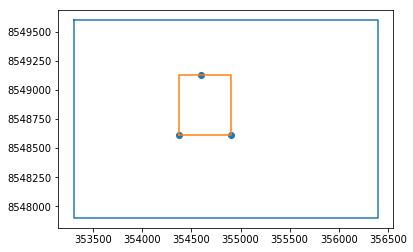
#Since we have geospatial and georeferenced data, we can add a satellite image in the background with the Mplleaflet package

import mplleaflet

crs = {'init' :'epsg:32718'}
mplleaflet.display(fig,crs=crs)

E:\Software\Anaconda37\lib\site-packages\IPython\core\display.py:689: UserWarning: Consider using IPython.display.IFrame instead
  warnings.warn("Consider using IPython.display.IFrame instead")
# Coordinates of the global and local discretization
GloRefBox = modelLimitShp.bbox
LocRefBox = modelWelShp.bbox
print(GloRefBox)
print(LocRefBox)
[353300.0, 8547900.0, 356400.0, 8549600.0]
[354369.8840337161, 8548609.34745342, 354904.6274241918, 8549128.04875159]
#Calculating Global Model (Glo) and Local Refinement (Loc) dimensions
GloLx = GloRefBox[2] - GloRefBox[0] #x_max - x_min
GloLy = GloRefBox[3] - GloRefBox[1]
print('Global Refinement Dimension. Easting Dimension: %8.1f, Northing Dimension: %8.1f' % (GloLx,GloLy))
LocLx = LocRefBox[2] - LocRefBox[0] #x_max - x_min
LocLy = LocRefBox[3] - LocRefBox[1]
print('Local Refinement Dimension. Easting Dimension: %8.1f, Northing Dimension: %8.1f' % (LocLx,LocLy))
Global Refinement Dimension. Easting Dimension: 3100.0, Northing Dimension: 1700.0
Local Refinement Dimension. Easting Dimension: 534.7, Northing Dimension: 518.7
#Defining Global and Local Refinements, for purpose of simplicity cell x and y dimension will be the same
celGlo = 100
celRef = 50
def arrayGeneratorCol(gloRef, locRef, gloSize, locSize):
cellArray = np.array([])
while cellArray.sum() + gloRef[0] < locRef[0] - celGlo:
cellArray = np.append(cellArray,[gloSize])
while cellArray.sum() + gloRef[0] > locRef[0] - celGlo and cellArray.sum() + gloRef[0] < locRef[2] + celGlo:
cellArray = np.append(cellArray,[locSize])
while cellArray.sum() + gloRef[0] > locRef[2] + celGlo and cellArray.sum() + gloRef[0] < gloRef[2]:
cellArray = np.append(cellArray,[gloSize])
return cellArray
def arrayGeneratorRow(gloRef, locRef, gloSize, locSize):
cellArray = np.array([])
accumCoordinate = gloRef[3] - cellArray.sum()
while gloRef[3] - cellArray.sum() > locRef[3] + celGlo:
cellArray = np.append(cellArray,[gloSize])
while gloRef[3] - cellArray.sum() < locRef[3] + celGlo and gloRef[3] - cellArray.sum() > locRef[1] - celGlo:
cellArray = np.append(cellArray,[locSize])
while gloRef[3] - cellArray.sum() < locRef[1] - celGlo and gloRef[3] - cellArray.sum() > gloRef[1]:
cellArray = np.append(cellArray,[gloSize])
return cellArray
#Remember that DELR is space between rows, so it is the column dimension array
delRArray = arrayGeneratorCol(GloRefBox, LocRefBox, celGlo, celRef)
delRArray
array([100., 100., 100., 100., 100., 100., 100., 100., 100., 100., 50.,
50., 50., 50., 50., 50., 50., 50., 50., 50., 50., 50.,
50., 50., 50., 100., 100., 100., 100., 100., 100., 100., 100.,
100., 100., 100., 100., 100., 100.])
#And DELC is the space between columns, so its the row dimension array
delCArray = arrayGeneratorRow(GloRefBox, LocRefBox, celGlo, celRef)
delCArray
array([100., 100., 100., 100., 50., 50., 50., 50., 50., 50., 50.,
50., 50., 50., 50., 50., 50., 50., 100., 100., 100., 100.,
100., 100.])
#Calculating number or rows and cols since they are dependant from the discretization
nrows = delCArray.shape[0]
ncols = delRArray.shape[0]
print('Number of rows: %d and number of cols: %d' % (nrows,ncols))
Number of rows: 24 and number of cols: 39
#Define some parametros and values for the spatial and temporal discretization (DIS package)
#Number of layers and layer elevations
nlays = 3
mtop = 0
botm = [-10,-20,-30]
#Number of stress periods and time steps
#In this case we will simulate the effect on the aquifer of 2000 days divided in 10 stress periods of 200 days,
#each stress period is divided in 4 time steps
#there is a steady state stress period at the beginning of the simulation
nper = 11
perlen = np.ones(nper)
perlen[0] = 1
perlen[1:] = 200 * 86400
#Definition of time steps
nstp = np.ones(11)
nstp[0] = 1
nstp[1:] = 4
#Definition of stress period type, transient or steady state
periodType = np.zeros(11, dtype=bool)
periodType[0] = True
print('This is the lenght of stress periods: ', perlen)
print('This is the number of time steps: ', nstp)
print('This is the stress period type: ', periodType)
This is the lenght of stress periods: [1.000e+00 1.728e+07 1.728e+07 1.728e+07 1.728e+07 1.728e+07 1.728e+07
1.728e+07 1.728e+07 1.728e+07 1.728e+07]
This is the number of time steps: [1. 4. 4. 4. 4. 4. 4. 4. 4. 4. 4.]
This is the stress period type: [ True False False False False False False False False False False]
# Apply the spatial and temporal discretization parameters to the DIS package
dis = flopy.modflow.ModflowDis(mf, nlay=nlays,
nrow=delCArray.shape[0],ncol=delRArray.shape[0],
delr=delRArray,delc=delCArray,
top=mtop,botm=botm,
itmuni=1.,nper=nper,perlen=perlen,nstp=nstp,steady=periodType)
#Assign spatial reference
mf.dis.sr = SpatialReference(delr=delRArray,delc=delCArray, xul=GloRefBox[0], yul= GloRefBox[3],epsg=32718)
mf.dis.sr.epsg
32718
mf.modelgrid.set_coord_info(xoff=GloRefBox[0], yoff=GloRefBox[3]-delCArray.sum(), angrot=0,epsg=32717)
fig = plt.figure(figsize=(8,8))
ax = fig.add_subplot(1, 1, 1, aspect='equal')
modelmap = flopy.plot.PlotMapView(model=mf)
linecollection = modelmap.plot_grid(linewidth=0.5, color='royalblue')
#Representation of model geometry with all the boundary conditions
fig = plt.figure(figsize=(8,8))

modelmap = flopy.plot.PlotMapView(model=mf)
linecollection = modelmap.plot_grid(linewidth=0.5, color='cyan')
shpRiver = flopy.plot.plot_shapefile('../Shp/ModelRiver2', facecolor='none') #RIV boundary condition
shpGHB = flopy.plot.plot_shapefile('../Shp/ModelGHB1', facecolor='none')     #GHB boundary condition

plt.plot(limitArray[:,0],limitArray[:,1])
plt.scatter(wellArray[:,0],wellArray[:,1])

crs = {'init' :'epsg:32718'}
mplleaflet.display(fig,crs=crs)
Definition of Model Top and Layer Bottom Elevation for the UPW package
dem = pd.read_csv('../Rst/ModeloDem2.csv')
dem.head()| Easting | Northing | Elevation | |
|---|---|---|---|
| 0 | 353214.799 | 8549716.14 | 58.925 |
| 1 | 353245.085 | 8549716.14 | 59.267 |
| 2 | 353275.372 | 8549716.14 | 59.609 |
| 3 | 353305.658 | 8549716.14 | 59.951 |
| 4 | 353335.945 | 8549716.14 | 60.293 |
points = dem[['Easting','Northing']].values
values = dem['Elevation'].values
grid_x = mf.modelgrid.xcellcenters
grid_y = mf.modelgrid.ycellcenters
mtop = griddata(points, values, (grid_x, grid_y), method='nearest')
mtop[:5,:5]

array([[60.293, 61.661, 62.686, 63.712, 65.08 ],
       [60.293, 61.661, 62.686, 63.712, 65.08 ],
       [60.293, 61.661, 62.686, 63.712, 65.08 ],
       [60.293, 61.661, 62.686, 63.712, 65.08 ],
       [60.293, 61.661, 62.686, 63.712, 65.08 ]])

fig = plt.figure(figsize=(8, 8))
ax = fig.add_subplot(1, 1, 1)
ax.set_aspect('equal')
modelmap = flopy.plot.PlotMapView(model=mf,ax=ax)
quadmesh = modelmap.plot_array(mtop)
#Asign surface elevations
mf.dis.top  = mtop

AcuifInf_Bottom = -120

AcuifMed_Bottom = AcuifInf_Bottom + (0.5 * (mtop - AcuifInf_Bottom))

AcuifSup_Bottom = AcuifInf_Bottom + (0.75 * (mtop - AcuifInf_Bottom))

zbot = np.zeros((nlays,nrows,ncols))

zbot[0,:,:] = AcuifSup_Bottom
zbot[1,:,:] = AcuifMed_Bottom
zbot[2,:,:] = AcuifInf_Bottom

#Asign layer bottom elevations
mf.dis.botm = zbot
fig = plt.figure(figsize=(20, 3))
ax = fig.add_subplot(1, 1, 1)
modelxsect = flopy.plot.PlotCrossSection(model=mf, line={'Row': 20})
linecollection = modelxsect.plot_grid()
Kx = np.zeros((nlays,nrows,ncols))
Kx[0,:,:] = 1E-5 #first layer of lime
Kx[1,:,:] = 5E-4 #second layer of sand
Kx[2,:,:] = 2E-4 #third layer of sandy gravel
fig = plt.figure(figsize=(20, 3))
ax = fig.add_subplot(1, 1, 1)
modelxsect = flopy.plot.PlotCrossSection(model=mf, line={'Row': 20})
linecollection = modelxsect.plot_grid()
modelxsect.plot_array(Kx)
print(Kx[:,10,10]) #print values of K for all layers in cell row / col = 10 , 10[1.e-05 5.e-04 2.e-04]
# Definition of layer type, the first two layers are convertible
laytyp = [1,1,0]
#lpf = flopy.modflow.ModflowLpf(mf, laytyp = laytyp, hk = Kx)
upw = flopy.modflow.ModflowUpw(mf, laytyp = laytyp, hk = Kx,
                              ss=1e-05, sy=0.15)
Configuration of active zones and initial heads: BAS package
ibound  = np.ones([nlays,nrows,ncols])
bas = flopy.modflow.ModflowBas(mf, ibound=ibound,strt=mtop)
Definition of the GRIDGEN object
For the manipulation of spatial data to determine hydraulic parameters or boundary conditions
g = Gridgen(mf.dis, model_ws=model_ws,exe_name='../Exe/gridgen_x64.exe',surface_interpolation='replicate')
g.build(verbose=False)
Recharge and Evapotranspiration as RCH and EVT boundary condition
# We apply recharge to the extension of the irrigated areas and evapotranspiration to the whole extent,
# The recharge rate is estimated in 200 mm /yr and the potential evapotraspiration is 1200 mm/yr

# Evapotranspiration rate
evtr = 1.2 / 365. / 86400. # 1200 mm/yr in m/s
evt = flopy.modflow.ModflowEvt(mf,evtr=evtr, surf=mtop, exdp=0.5, nevtop=1)
# Recharge rate
rechRate = 0.2 / 365. / 86400. # 200 mm/yr in m/s
rech_intersect = g.intersect('../Shp/ModelRechargeZone1','polygon',0)
rech_spd = {} # empty dictionary for all stress periods, actually spd comes from stress period data
rech_spd[0] = np.zeros([nrows,ncols]) # empty list as the first item of dictionary for the first stress period
rech_unique = np.unique(rech_intersect.nodenumber) # unique cells where recharge is applied, the np.unique also sorts the cell number
print(rech_unique[:5]) # a sample of the sorted list[0 1 2 3 4]for i in np.arange(rech_unique.shape[0]):
x,y = g.get_center(rech_unique[i]) #get the cell centroid x and y
i,j = mf.sr.get_ij(x,y) #get the cell row and column
rech_spd[0][i,j] =rechRate #add the recharge in the cell to the array for the first stress period
# Recharge is applied to the highest active cell nrchop = 3 (default)
rec = flopy.modflow.ModflowRch(mf, nrchop=3, rech=rech_spd)# Representation of applied recharge values for the last stress period.
# For flopy, and modflow if no recharge for other stress period is specified, the first recharge will remain for the entire simulation.
fig = plt.figure(figsize=(12, 12))
ax = fig.add_subplot(1, 1, 1, aspect='equal')
modelmap = flopy.plot.PlotMapView(model=mf)
quadmesh = modelmap.plot_array(mf.rch.rech.array[-1,0,:,:], alpha=0.3)
wel_intersect = g.intersect('../Shp/ModelWell2','point',0)
wel_spd = {}
wel_spd[0] = [0,0,0,0] #wells are not pumping on steady state (stress period 1) but we have to insert zero pumping rate to at least one cells
wel_spd[1] = []
wel_unique = np.unique(wel_intersect.nodenumber) #For the well case this is kind of redundant because wells are located apart form each other
#It could be good if the shapefile have overlying points
for i in np.arange(wel_unique.shape[0]):
    x,y = g.get_center(wel_unique[i])
    i,j = mf.sr.get_ij(x,y)
    wel_spd[1].append([1,i,j,-0.03]) #well are located on the second layer and each of them pump 10 l/s (-0.001 m3/s)
wel = flopy.modflow.ModflowWel(mf,stress_period_data=wel_spd)# Plot the well shapefile and the cells conceptualized as wells
fig = plt.figure(figsize=(12, 12))
ax = fig.add_subplot(1, 1, 1, aspect='equal')
modelmap = flopy.plot.PlotMapView(model=mf)
g.plot(ax, linewidth=0.5)
quadmesh = modelmap.plot_array(mf.wel.stress_period_data.array['flux'][-1,1,:,:], cmap='Spectral',ax=ax)
shp = flopy.plot.plot_shapefile('../Shp/ModelWell2', ax=ax, radius=10)
River path as RIV boundary condition
river_intersect = g.intersect('../Shp/ModelRiver2', 'polygon', 0)
river_spd = {}
river_spd[0] = []
river_unique = np.unique(river_intersect.nodenumber)
for i in np.arange(river_unique.shape[0]):
    x,y = g.get_center(river_unique[i])                           # river_intersect.nodenumber[i]
    i,j = mf.sr.get_ij(x, y)
    river_spd[0].append([0,i,j,mtop[i,j],0.01,mtop[i,j]-1])         # the array follow this order: [lay, row, col, stage, cond, rbot]
riv = flopy.modflow.ModflowRiv(mf, stress_period_data=river_spd)# Plot the river shapefile and the cells conceptualized as river
fig = plt.figure(figsize=(12, 12))
ax = fig.add_subplot(1, 1, 1, aspect='equal')
modelmap = flopy.plot.PlotMapView(model=mf)
g.plot(ax, linewidth=0.5)
quadmesh = modelmap.plot_array(mf.riv.stress_period_data.array['cond'][-1,0,:,:], cmap='Spectral',ax=ax, alpha=0.5)
shp = flopy.plot.plot_shapefile('../Shp/ModelRiver2', ax=ax,facecolor='none')
Regional flow as GHB boundary condition
ghb_intersect = g.intersect('../Shp/ModelGHB1', 'line', 0)
ghb_spd = {}
ghb_spd[0] = []
ghb_unique = np.unique(ghb_intersect.nodenumber)
ghb_unique
array([ 0, 38, 39, 77, 78, 116, 117, 155, 156, 194, 195, 233, 234,
272, 273, 312, 351, 390, 429, 506, 545, 584, 623, 662, 663, 701,
702, 740, 741, 779, 780, 818, 819, 857, 858, 896, 897, 935])for i in np.arange(ghb_unique.shape[0]):
x,y = g.get_center(ghb_unique[i]) # river_intersect.nodenumber[i]
i,j = mf.sr.get_ij(x, y)
if j < 5:
ghb_spd[0].append([0,i,j,55,0.01]) # the array follow this order: [lay, row, col, elev, cond]
elif j > ncols -5:
ghb_spd[0].append([0,i,j,90,0.01])
else: print("GHB on the wrong position")ghb = flopy.modflow.ModflowGhb(mf, stress_period_data=ghb_spd)# Plot the GHB shapefile and the cells conceptualized as GHB
fig = plt.figure(figsize=(12, 12))
ax = fig.add_subplot(1, 1, 1, aspect='equal')
modelmap = flopy.plot.PlotMapView(model=mf)
g.plot(ax, linewidth=0.5)
quadmesh = modelmap.plot_array(mf.ghb.stress_period_data.array['cond'][-1,0,:,:], cmap='RdGy',ax=ax, alpha=0.2)
shp = flopy.plot.plot_shapefile('../Shp/ModelGHB1', ax=ax,linewidth=8)
### Set the Output Control and run simulationoc_spd = {(0, 0): ['save head']}
for i in range(mf.dis.nstp.shape[0]):
oc_spd[(i,mf.dis.nstp.array[3]-1)] = ['save head']
oc_spd{(0, 0): ['save head'],
(0, 3): ['save head'],
(1, 3): ['save head'],
(2, 3): ['save head'],
(3, 3): ['save head'],
(4, 3): ['save head'],
(5, 3): ['save head'],
(6, 3): ['save head'],
(7, 3): ['save head'],
(8, 3): ['save head'],
(9, 3): ['save head'],
(10, 3): ['save head']}oc = flopy.modflow.ModflowOc(mf, stress_period_data=oc_spd)mf.write_input()
mf.run_model()FloPy is using the following executable to run the model: ../Exe/MODFLOW-NWT_64.exe
MODFLOW-NWT-SWR1
U.S. GEOLOGICAL SURVEY MODULAR FINITE-DIFFERENCE GROUNDWATER-FLOW MODEL
WITH NEWTON FORMULATION
Version 1.1.4 4/01/2018
BASED ON MODFLOW-2005 Version 1.12.0 02/03/2017
SWR1 Version 1.04.0 09/15/2016
Using NAME file: Model1.nam
Run start date and time (yyyy/mm/dd hh:mm:ss): 2019/06/10 10:57:55
Solving: Stress period: 1 Time step: 1 Groundwater-Flow Eqn.
Solving: Stress period: 2 Time step: 1 Groundwater-Flow Eqn.
Solving: Stress period: 2 Time step: 2 Groundwater-Flow Eqn.
Solving: Stress period: 2 Time step: 3 Groundwater-Flow Eqn.
Solving: Stress period: 2 Time step: 4 Groundwater-Flow Eqn.
Solving: Stress period: 3 Time step: 1 Groundwater-Flow Eqn.
Solving: Stress period: 3 Time step: 2 Groundwater-Flow Eqn.
Solving: Stress period: 3 Time step: 3 Groundwater-Flow Eqn.
Solving: Stress period: 3 Time step: 4 Groundwater-Flow Eqn.
Solving: Stress period: 4 Time step: 1 Groundwater-Flow Eqn.
Solving: Stress period: 4 Time step: 2 Groundwater-Flow Eqn.
Solving: Stress period: 4 Time step: 3 Groundwater-Flow Eqn.
Solving: Stress period: 4 Time step: 4 Groundwater-Flow Eqn.
Solving: Stress period: 5 Time step: 1 Groundwater-Flow Eqn.
Solving: Stress period: 5 Time step: 2 Groundwater-Flow Eqn.
Solving: Stress period: 5 Time step: 3 Groundwater-Flow Eqn.
Solving: Stress period: 5 Time step: 4 Groundwater-Flow Eqn.
Solving: Stress period: 6 Time step: 1 Groundwater-Flow Eqn.
Solving: Stress period: 6 Time step: 2 Groundwater-Flow Eqn.
Solving: Stress period: 6 Time step: 3 Groundwater-Flow Eqn.
Solving: Stress period: 6 Time step: 4 Groundwater-Flow Eqn.
Solving: Stress period: 7 Time step: 1 Groundwater-Flow Eqn.
Solving: Stress period: 7 Time step: 2 Groundwater-Flow Eqn.
Solving: Stress period: 7 Time step: 3 Groundwater-Flow Eqn.
Solving: Stress period: 7 Time step: 4 Groundwater-Flow Eqn.
Solving: Stress period: 8 Time step: 1 Groundwater-Flow Eqn.
Solving: Stress period: 8 Time step: 2 Groundwater-Flow Eqn.
Solving: Stress period: 8 Time step: 3 Groundwater-Flow Eqn.
Solving: Stress period: 8 Time step: 4 Groundwater-Flow Eqn.
Solving: Stress period: 9 Time step: 1 Groundwater-Flow Eqn.
Solving: Stress period: 9 Time step: 2 Groundwater-Flow Eqn.
Solving: Stress period: 9 Time step: 3 Groundwater-Flow Eqn.
Solving: Stress period: 9 Time step: 4 Groundwater-Flow Eqn.
Solving: Stress period: 10 Time step: 1 Groundwater-Flow Eqn.
Solving: Stress period: 10 Time step: 2 Groundwater-Flow Eqn.
Solving: Stress period: 10 Time step: 3 Groundwater-Flow Eqn.
Solving: Stress period: 10 Time step: 4 Groundwater-Flow Eqn.
Solving: Stress period: 11 Time step: 1 Groundwater-Flow Eqn.
Solving: Stress period: 11 Time step: 2 Groundwater-Flow Eqn.
Solving: Stress period: 11 Time step: 3 Groundwater-Flow Eqn.
Solving: Stress period: 11 Time step: 4 Groundwater-Flow Eqn.
Run end date and time (yyyy/mm/dd hh:mm:ss): 2019/06/10 10:57:55
Elapsed run time: 0.242 Seconds
Normal termination of simulation
(True, [])Model output visualization
mfheads = flopy.utils.HeadFile('../Model/Model1.hds')
mfheads.get_times()
[1.0,
17280000.0,
34560000.0,
51840000.0,
69120000.0,
86400000.0,
103680000.0,
120960000.0,
138240000.0,
155520000.0,
172800000.0]head = mfheads.get_data()
head.shape(3, 24, 39)# Plot the heads for a defined layer and boundary conditions
fig = plt.figure(figsize=(36, 24))
ax = fig.add_subplot(1, 1, 1, aspect='equal')
modelmap = flopy.plot.PlotMapView(model=mf)
g.plot(ax, linewidth=0.5, alpha=0.4)
contour = modelmap.contour_array(head[1],ax=ax)
quadmesh = modelmap.plot_array(mf.riv.stress_period_data.array['cond'][-1,0,:,:], cmap='Spectral',ax=ax, alpha=0.5)
cellhead = modelmap.plot_array(head[1],ax=ax, cmap='Blues', alpha=0.2)
ax.clabel(contour)
plt.tight_layout()
# Boundary conditions
shpGHB = flopy.plot.plot_shapefile('../Shp/ModelGHB1', ax=ax,linewidth=8)
shpWel = flopy.plot.plot_shapefile('../Shp/ModelWell2', ax=ax,radius=20)
shpRiv = flopy.plot.plot_shapefile('../Shp/ModelRiver2', ax=ax)
# Export heads on layer two at the beggining of simulation
contourShp = mfheads.to_shapefile(filename='../Shp/ModelHeadsLay2',kstpkper=(0,0),mflay=1)
fig.savefig('infahatari.png')wrote ../Shp/ModelHeadsLay2
#Representation of model geometry with all the boundary conditions
fig = plt.figure(figsize=(18,8))

modelmap = flopy.plot.PlotMapView(model=mf)
linecollection = modelmap.plot_grid(linewidth=0.5, color='cyan')
shpRiver = flopy.plot.plot_shapefile('../Shp/ModelRiver2', facecolor='none') #RIV boundary condition
shpGHB = flopy.plot.plot_shapefile('../Shp/ModelGHB1', facecolor='none')     #GHB boundary condition

contour = modelmap.contour_array(head[1])
plt.plot(limitArray[:,0],limitArray[:,1])
plt.scatter(wellArray[:,0],wellArray[:,1])

tiles=('http://mt0.google.com/vt/lyrs=s&hl=en&x={x}&y={y}&z={z}',
       '<a href=https://www.openstreetmap.org/about">© OpenStreetMap</a>')
crs = {'init' :'epsg:32718'}
mplleaflet.display(fig, crs=crs, tiles=tiles)
fig = plt.figure(figsize=(20, 3))
ax = fig.add_subplot(1, 1, 1)
modelxsect = flopy.plot.PlotCrossSection(model=mf, line={'Row': 10})
linecollection = modelxsect.plot_grid()
modelxsect.contour_array(head)Input data
Download the input data for this tutorial here.