
Interactive visualization of aquifer response to pumping with MODFLOW6, Flopy and Jupyter
/
Aquifer response to pumping is one of the most popular interactions between human and the groundwater flow regimen. On the complexity of the hydrogeological studies, pumping tests are the most controlled environments since the well construction details are known, geological logs are available and pumping rates and drawndows can be measured. There are uncertainties on this hydraulic test and these are mostly related to the aquifer heterogeneity, however, it is expected that a pumping test can be fully recreated on a numerical model.
MODFLOW is the groundwater flow model developed by the USGS based on finite differences (regular grids). MODFLOW works on a DOS terminal, there are commercial/free software for the pre and postprocessing of groundwater models on MODFLOW. Some of these software perform animations of the groundwater heads development, however, the available tools to create custom animations that interact with user inputs /options are limited.
Flopy is the Python library to build, run and post-process MODFLOW models, including the latest MODFLOW version: MODFLOW 6. Jupyter is a interactive computational environment that combine Python code and output representation. Flopy and Jupyter together can provide new and powerful ways to analyze the hydrogeological response to a pumping test on a numerical model. The use of a interactive HTML widgets on Jupyter as sliders allow the user to go back and forth on the time steps, enhancing the understanding of the water table and groundwater heads development.
Animation
This is a cross section of the aquifer response to pumping on the center cell

Tutorial
Input data
You can download the required data for this tutorial here.
Python code
This is the full Python code for the tutorial:
Import required packages for simulation and representation
import os, flopy, sys
import matplotlib.pyplot as plt
import numpy as np
import pandas as pd
Definition of Simulation Names and Model Names
MODFLOW 6 can model the interaction among different models, that is why a simulation and model has to be created. This simulation/model concept seems complicated for a beginner user, and so far we havent done any simulation with model exchange.
exampleDir = os.path.dirname(os.getcwd())
simName = 'model41x41sim'
simPath = exampleDir + '\Simulation'
exeName = exampleDir + '\Exe\mf6.exe'

sim = flopy.mf6.MFSimulation(sim_name=simName,
                             version='mf6', exe_name=exeName,
                             sim_ws=simPath)
Model creation and solver options
For this tutorial we have used the GWF Model of MODFLOW 6, that is the only available in Flopy. The GWF Model adopts the Newton-Raphson formulation, the same formulation implemented in MODFLOW NWT. This solver is powerful when dealing with complex geometries and discretizations.
modelName='model41x41well'
model = flopy.mf6.MFModel(sim,modelname=modelName,model_nam_file=modelName+'.nam')
#creation of a Iterative Model Solution (IMS)
imsPackage = flopy.mf6.ModflowIms(sim, print_option='ALL',
                                   complexity='SIMPLE', outer_hclose=0.00001,
                                   outer_maximum=50, under_relaxation='NONE',
                                   inner_maximum=30, inner_hclose=0.00001,
                                   linear_acceleration='CG',
                                   preconditioner_levels=7,
                                   preconditioner_drop_tolerance=0.01,
                                   number_orthogonalizations=2)
#register solution to the sim
sim.register_ims_package(imsPackage,[modelName])
Temporal and spatial discretization
Model has 2 stress periods (nper) of 10 days divided into 10 time steps. Time unit for this model is seconds and spatial unit is meters. All the model parameters were inserted in a combination of this units. Spatial discretization is regular. On the horizontal plane, each cell has a with of 1m. Each layer has a thickness of 2m.
# Temporal discretization in MODFLOW 6
tdis = flopy.mf6.ModflowTdis(sim, time_units='SECONDS', nper=2,
                            perioddata=((864000.0, 10, 1.2),
                                        (864000.0, 10, 1.2)))
modelCells = 101
cellSize = 1

# Spatial discretization in MODFLOW 6
discListModel = []
for cell in range(modelCells):
    discListModel.append(cellSize)

bottoms=[]
for a in range(30):
    bottoms.append(100-2*a-2)
print(bottoms)

disPackage = flopy.mf6.ModflowGwfdis(model, length_units='METERS',
                                    nlay=30, nrow=modelCells, ncol=modelCells,
                                     delr=discListModel, delc=discListModel,
                                     top =100, botm=bottoms)
Hydraulic conductivity definition
The well cell and all the cells above have increased K of 10 m/s.
K = 3e-5
kArray = np.ones([30,modelCells,modelCells])*K
kArray[:20,50,50]=1
npfPackage = flopy.mf6.ModflowGwfnpf(model, save_flows=True, icelltype=1, k=kArray)
Initial heads and storage parameter definition
All layers are convertible, that means they can be confined or unconfined upon difference between cell top and water head.
# Initial conditions
icPackage = flopy.mf6.ModflowGwfic(model,strt=99)

# Storage parameters
genSs = 1e-5
genSy = 0.10

#define dynamic hydraulic parameters, the first layer is convertible and the second is confined
stoPackage = flopy.mf6.ModflowGwfsto(model, save_flows=True, iconvert=1,
                                     ss=genSs, sy=genSy,
                                     transient=True) #
Boundary condition definition (CHD and Well)
Two boundary conditions were conceptualized for this model. The constant head boundary was inserted with the values of the initial heads. The CHDs located at the model borders on the first 10 layers to give more numerical stability and improve model convergence. Pumping on the WEL package cell is 12 l/s on the first 10 days and 18 l/s on the second stress period.Pumping was distributed in 5 layers.
# CHD package
chdList = []
for cell in range(modelCells):
    for lay in range(10):
        chdList.append([[lay,cell,0],99])
        chdList.append([[lay,cell,100],99])

CHD_data = {0:chdList}
chdPackage = flopy.mf6.ModflowGwfchd(model, stress_period_data=CHD_data)

# Well package
welData = {0:[[[15,50,50],-0.012/5],
              [[16,50,50],-0.012/5],
              [[17,50,50],-0.012/5],
              [[18,50,50],-0.012/5],
              [[19,50,50],-0.012/5]],
           1:[[[15,50,50],-0.018/5],
              [[16,50,50],-0.018/5],
              [[17,50,50],-0.018/5],
              [[18,50,50],-0.018/5],
              [[19,50,50],-0.018/5]],
          }

# build the well package
welPackage = flopy.mf6.ModflowGwfwel(model, stress_period_data=welData, boundnames=True, save_flows=True)
Output controls and simulation
#set up Output Control Package
printrec_tuple_list = [('BUDGET', 'ALL')]
saverec_dict = [('HEAD', 'ALL'),('BUDGET', 'ALL')]
ocPackage = flopy.mf6.ModflowGwfoc(model,
                                   budget_filerecord=[modelName+'.cbc'],
                                   head_filerecord=[modelName+'.hds'],
                                   saverecord=saverec_dict,
                                    printrecord=printrec_tuple_list)

# Simulation and run
sim.write_simulation()
sim.run_simulation()
Output representation
We open model results and make a interactive representation of the water table development.
# get all head data
totalHeads = sim.simulation_data.mfdata[modelName, 'HDS', 'HEAD']

def waterTable(selHead):
    wtHeads = np.zeros([modelCells,modelCells])
    for row in range(modelCells):
        for col in range(modelCells):
            heads=selHead[:,row,col]
            wtHeads[row,col]=heads[heads>1][0]
    return wtHeads
import matplotlib.patches as pch
def plotCrossSection(selTime):
# get selected heads
selHead = totalHeads[selTime]
# get Water Table data
wtHeads = waterTable(selHead)
extent = (0, 101, 40, 100)
fig = plt.figure(figsize=(30,20))
ax = plt.subplot(111)
cax = ax.imshow(selHead[:,20,:], interpolation='nearest', cmap=plt.cm.Blues,
extent=extent,vmin=90)
fig.colorbar(cax, format = '%.1f',orientation="horizontal", pad=0.03,shrink=0.5)
cellCenterArray = np.linspace(0.5,100.5,modelCells)
ax.plot(cellCenterArray,wtHeads[50,:],color='orange')
ax.add_patch(pch.Rectangle((50,60),1,40, color=(0.4, 0.4, 0.5)))import ipywidgets as widgets
widgets.interact(plotCrossSection,
selTime=widgets.IntSlider(
value=0,
min=0,
max=totalHeads.shape[0]-1,
description = 'Time (days):',
step=1))