Discretization is the “art” of transforming a continuous media as nature into discrete parts; for numerical models the spatial and temporal discretization have become a key issue in assuring model efficiency, output precision and the overall quality of the modeling work. Flow models are constructed to represent an specific requirement on the surface water/ groundwater flow regime (local scale), however, the model has to represent first the overall flow regimen (global scale). On the general model areas, an efficient spatial discretization criteria rules to keep the mesh elements as big as possible, meanwhile, in the areas of interest the model should be discretized into the smallest parts.

The discretization runs a paradox on the model mesh construction: the model mesh can't be so fine because it would require lots of computational power among other resources; and as long as the discretization increases the cell size, the model will lose resolution. The right balance in between precision/computational power come from the modelers experience and model objectives; that is why we call discretization an “art” since every modeler will use a different discretization schema to represent nature as artist choose colors and brushes to paint objects.

In OpenFOAM we cannot talk about a grid, instead we have to use a mesh since the tetrahedra are not exactly aligned on a layer. Numerical mesh for OpenFOAM models can be done through build in OpenFOAM tools as BlockMesh or SnappyHexMesh or with the use of third party software as Salome Platform. The number and size of tetrahedra can be relevant in the following aspects of the model simulation.

Output file sizes
Model resolution
Simulation time step (related to the Courant number)
Visualization software performance

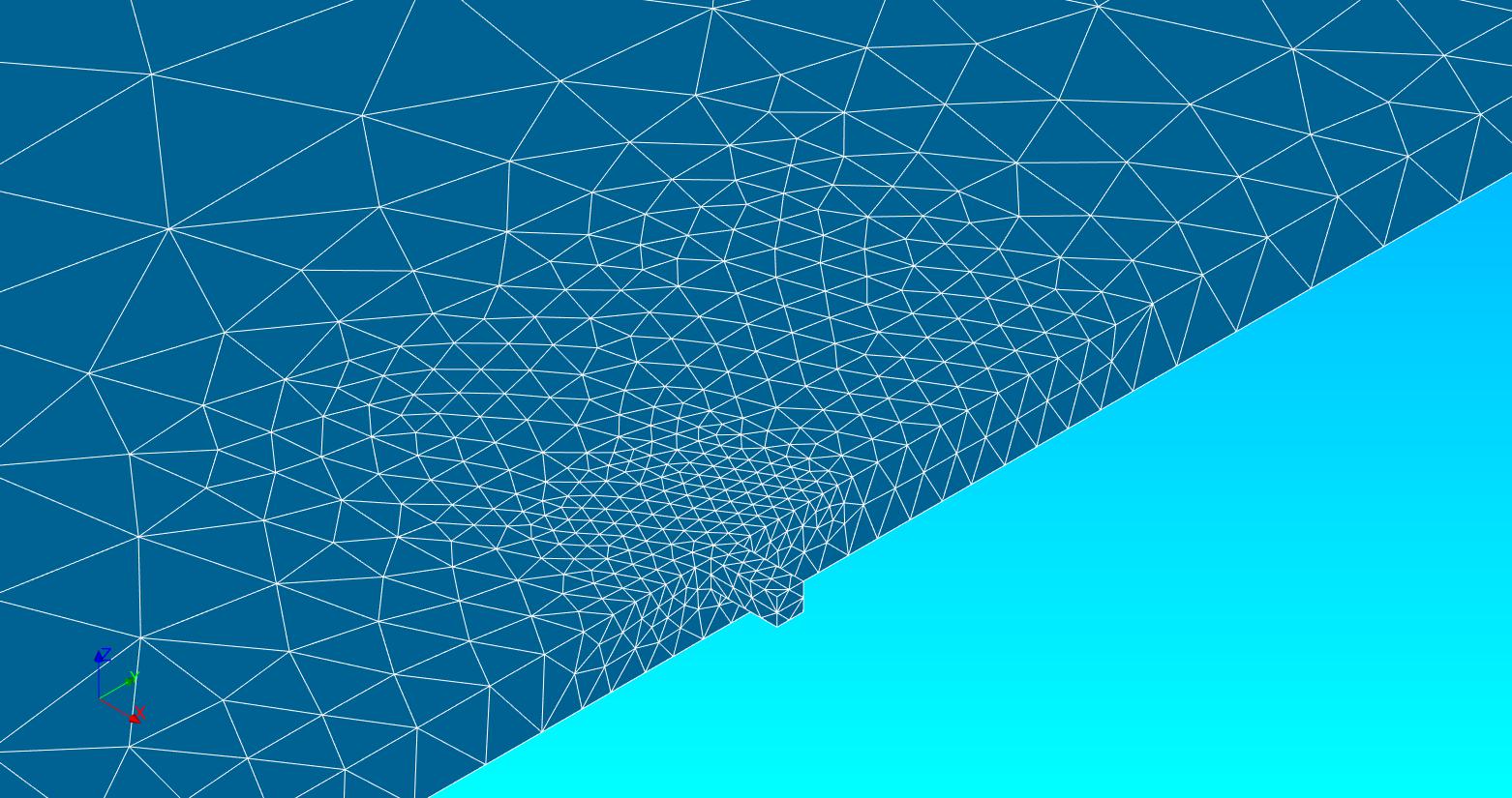
Tetrahedral mesh in Salome Platform

Salome Platform is a software for pre and post visualization of numerical models. It has several options for grid and mesh creation and some of them are compatible with OpenFOAM. By default the mesh size is related with the model vertex, edge length and default parameters from the software. There is chance to improve the mesh with refinement by face, vertex or edge, however this approach is sometimes limited to represent the flow regime with accurate precision.

Another option is to use a mesh size file with extension “*.msz” to determine the maximum mesh size at the given points or specified lines. This approach is more useful when we try to have more elements in the area of interest and less elements outside this area.

The layout of a mesh size file is:

<num of points>
<x1> <y1> <z1> <maxH1>
<x2> <y2> <z2> <maxH2>
<x3> <y3> <z3> <maxH3>
...
...
...
...
<xN> <yN> <zN> <maxHN>

<num of lines>
<x11> <y11> <z11> <x12> <y12> <z12> <maxH1>
<x21> <y21> <z21> <x22> <y22> <z22> <maxH2>
<x31> <y31> <z31> <x32> <y32> <z32> <maxH3>
...
...
...
...
<xN1> <yN1> <zN1> <xN2> <yN2> <zN2> <maxHN>

Where the modeler give point coordinates or line edge coordinates and the given mesh size.

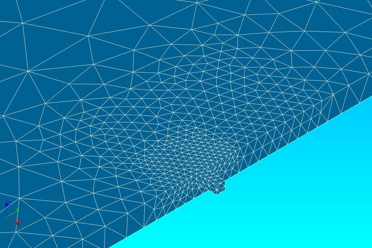
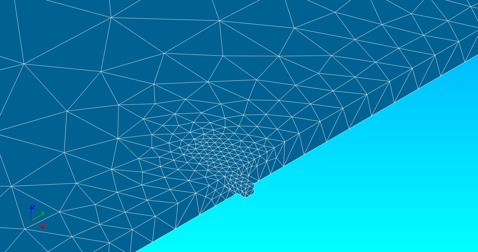
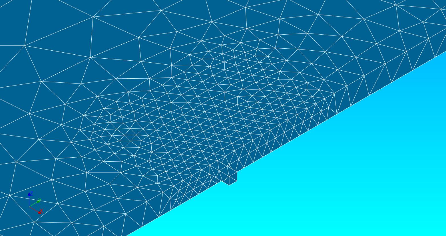
In 3D flow models with complex geometries we want to define regions for mesh refinement, then the point or line definition process is not so practical. In order to improve this, we have done a Python script that creates a model mesh file with hundreds of points at a given region and cell size. The script is very convenient since it allows to create progressive refinements on the model mesh.

Photo gallery

Default refiment

Handmade refinement

One stage refinement

Two stage refinement

Tutorial

Python code

Here is the python code for a single stage refinement, the script uses common numerical packages as Numpy and build in packages as Math. The code creates a msz file, define the number of points and point distribution along axis, then it writes the data on the file. Example of two stage refinement can be found in the input file part of this tutorial.

import numpy as np

import math

mszrect = open('../Txt/refinementStruc.msz','w')

#Refinement1

Ref1 = {

   'cellsize' : 0.4,

   'xinit' : 15,

   'xend' : 20,

   'yinit' : 8,

   'yend' : 16,

   'zinit' : -1,

   'zend' : 0

}

def pointsData(Ref):

   numberx = math.ceil((Ref['xend']-Ref['xinit'])/Ref['cellsize'])+1

   numbery = math.ceil((Ref['yend']-Ref['yinit'])/Ref['cellsize'])+1

   numberz = math.ceil((Ref['zend']-Ref['zinit'])/Ref['cellsize'])+1

   totalNumber = numberx*numbery*numberz

   xarray = np.linspace(Ref['xinit'],Ref['xend'],numberx)

   yarray = np.linspace(Ref['yinit'],Ref['yend'],numbery)

   zarray = np.linspace(Ref['zinit'],Ref['zend'],numberz)

   return [totalNumber, xarray, yarray, zarray]

def writeData(datosRef,Ref):

   for z in datosRef[3]:

       for x in datosRef[1]:

           for y in datosRef[2]:

               print(x, y, z)

               mszrect.write(str(x)+' '+str(y)+' '+str(z)+' '+str(Ref['cellsize'])+'\n')  

datosRef1 = pointsData(Ref1)

npoints = datosRef1[0]

mszrect.write(str(npoints)+'\n')

writeData(datosRef1,Ref1)

mszrect.write('0 \n')

mszrect.close()