Land Cover Change Analysis with Python and GDAL - Tutorial

Satellite imagery brought us the capacity to see the land surface on recent years but we haven’t been so successful to understand land cover dynamics and the interaction with economical, sociological and political factors. Some deficiencies were found on the use of GIS commercial software, but there are other limitations in the way we apply logical and mathematical processes to a set of satellite imagery. Working with geospatial data on Python gives us the capability to filter, calculate, clip, loop, and export raster or vector datasets with an efficient use of the computational power providing a bigger scope on data analysis.

This tutorial shows the complete procedure to create a land cover change raster from a comparison of generated vegetation index (NDVI) rasters by the use of Python and the Numpy and GDAL libraries. Contours of land cover change where generated with some tools of GDAL and Osgeo and an analysis of deforestation were done based on the output data and historical images from Google Earth.

Read More

1 Comment


Suscribe to our online newsletter

Subscribe for free newsletter, receive news, interesting facts and dates of our courses in water resources.


Stable Isotope Representation from Groundwater Samples with Python Pandas - Tutorial

Stable isotope analysis is a powerful tool for the evaluation of groundwater origin and groundwater dynamics, specially when the observation points and recording periods are limited. Isotope representation can be done with any spreadsheet software, but the workflow is defficient specially when plotting scatter points, solid lines, labels and legends.

This tutorial shows a the complete procedure to represent a stable isotope representation of groundwater samples from remediation site in New Mexico, USA. The script is done with Python 3, Pandas and other packages that come alread installed on the Anaconda distribution. Code for the representation of the Global Meteoric Water Line is also included as well as options for the figure storage.

Read More
4 Comments


Suscribe to our online newsletter

Subscribe for free newsletter, receive news, interesting facts and dates of our courses in water resources.


How to clip multiple Landsat 8 Bands with Python and GDAL - Tutorial

Current GIS desktop applications are fully capable of this spatial management and analysis when the amount of raster images is limited; however when we deal with high amount of images the spatial processing on a graphical user interfase (GUI) can be slow and most commonly impractical. The use of programming / processing languages like Python and advanced spatial libraries as GDAL (gdal.org) helps on the spatial data transformation on a more abstract and effective way. This tutorial shows the complete procedure to clip the complete set of bands from a Landsat 8 image and store them with a suffix on every band file on another folder.

The tutorial is done on a interactive Python programming platform called Jupyter Notebook. The input files: raster bands and area of interest (AOI) shapefile need to be on the same system of reference (SRC), otherwise the GDAL library cannot locate the spatial data on the right position. The tutorial shows the procedure for the whole set of band form a Landsat 8 image, an example for a single band is provided on the scripts of the input data. Finally the tutorial shows the complete and clipped raster on a GIS desktop software as QGIS.

Read More
5 Comments


Suscribe to our online newsletter

Subscribe for free newsletter, receive news, interesting facts and dates of our courses in water resources.


Regional Groundwater Modeling with MODFLOW and Flopy - Tutorial

Regional groundwater modeling is an important task on a strategic water management that involves all users, activities, and involved ecosystems and provides a sustainable use for current and future conditions. There are some specific considerations on the regional modeling with respect to baseline and spatial discretization, a regional model is not intended to provide the aquifer response for a determined area, instead it involves the assessment of the regional groundwater flow and the quantification of the recharge, discharge and other process on the water balance.

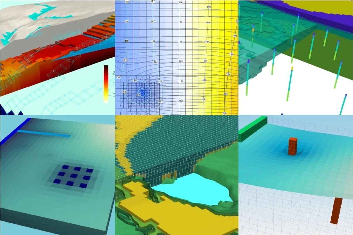
This tutorial is the Flopy / MODFLOW numerical example of the Angascancha basin. The example is on steady steady and is solved with the NWT solver. Model output representations have been done under the Flopy/Matplotlib tools as well as some Python code to create VTU files and styled on Paraview.

Read More


Suscribe to our online newsletter

Subscribe for free newsletter, receive news, interesting facts and dates of our courses in water resources.


Basic Example of Saline Intrusion Modeling with SEAWAT and Flopy - Tutorial

SEAWAT is a model developed by the USGS for the simulation of three-dimensional variable density groundwater flow with solute and heat transport. The software is based on MODFLOW-2000 and MT3DMS and on its latest version it can simulate viscosity variations and provide faster execution times. SEAWAT is implemented on Flopy, the Python library to build, run and represent MODFLOW models. This tutorial has the complete workflow to create and represent a basic example of saline instrusion with SEAWAT and Flopy on a Jupyter Notebook.

Read More


Suscribe to our online newsletter

Subscribe for free newsletter, receive news, interesting facts and dates of our courses in water resources.


Determination of Flow Direction Vectors from a MODFLOW Model with Python and Flopy - Tutorial

Groundwater flow direction representation is useful to understand the actual and predicted conditions of the groundwater flow regime. The arrow direction and magnitude give a quick perspective of the main groundwater flow directions and the interconexion between sources and discharge points. This tutorial show the complete workflow to determine the flow directions from a MODFLOW model done with Model Muse. The scripting insert a background image, georeference the model from parameters exported as comments, and export the resulting figure as a PNG file. The tutorial is done in Python 3 on a Jupyter Notebook.

Read More


Suscribe to our online newsletter

Subscribe for free newsletter, receive news, interesting facts and dates of our courses in water resources.


How to make a Piper Diagram in Python - Tutorial

A Piper Diagram is an effective graphic procedure to segregate relevant analytical data to understand the sources of the dissolved constituents in water. This procedure was born under the statement that most natural waters contain cations and anions in chemical equilibrium. It is assumed that the most abundant cations are calcium (Ca), magnesium (Mg) and sodium (Na). The most common anions are bicarbonate (HCO3), sulphate (SO4) and chloride (Cl).

The Piper diagram can be made by free and commercial desktop software, however in this tutorial we have generated the Python scripts and working procedure to create a Piper Diagram from values stored in a working spreadsheet.

Read More


Suscribe to our online newsletter

Subscribe for free newsletter, receive news, interesting facts and dates of our courses in water resources.


NDVI calculation from Landsat8 images with Python 3 and Rasterio - Tutorial

Satellite images are georasters, these images are a regular array of columns and rows (a matrix per band) with a georeferenciation. Python is a programming and data analysis language very versatile for the matrix algebra with the Numpy library, however there was no efective and simple way to process a georaster until the development of the Rasterio package.

Rasterio is a library to open, write, explore and analyze georasters in Python. The library uses GeoTIFF images along with other formats and is capable to work with satellite images, digital elevation models, and drone generated imagery.

This tutorial show the complete procedure to analyse the NDVI from a Landsat 8 image with Python 3 and Rasterio. The scripting and representation was performed on a interactive enviroment called Jupyter Notebook, finally the result georaster was opened in QGIS and compared with some background images.

Read More


Suscribe to our online newsletter

Subscribe for free newsletter, receive news, interesting facts and dates of our courses in water resources.


Sentinel2 images exploration and processing with Python and Rasterio - Tutorial

Rasterio is a Python library that allows to read, inspect, visualize and write geospatial raster data. The library uses GeoTIFF and other spatial raster formats and is capable of working with satellite imagery, digital elevation models, and drone imagery data products. Rasterio allows you to import a single band or multiband geospatial raster in a interactive Python enviroment as Jupyter notebook, the library can keep the “duality” of the geospatial raster, that means, it can handle the location and resolution parameters as well as the matrix values of the gridded elements.

This tutorial shows some basic procedures to explore a multiband Sentinel 2 granule with Python 3 and Rasterio on a Jupyter Notebook. The tutorial shows the commands to identify the raster array dimensions and the geospatial referencing parameters, make representation of each visible band and export band composites as true color and false color geoespatial rasters in Tiff format.

Read More


Suscribe to our online newsletter

Subscribe for free newsletter, receive news, interesting facts and dates of our courses in water resources.


Elevation Model Conditioning and Stream Network Delimitation with Python and Pysheds - Tutorial

Digital elevation models (DEMs) from satellite interpretation (Aster DEM or Alos Palsar) come with “sinks” from errors in the elevation interpretation, raster resolution or reprojection. There is a need to correct those rasters in order to interpret the hydrological features. This tutorial show the process to condition a digital elevation model (DEM) dowloaded from a NASA/USGS server (gdex.cr.usgs.gov) with the Pysheds library of Python. The tutorial was done on a Jupyter Notebook, input files and scripts are attached on the final part of the post.

Read More


Suscribe to our online newsletter

Subscribe for free newsletter, receive news, interesting facts and dates of our courses in water resources.


How to calculate a Terrain Volume with QGIS3 - Tutorial

Calculate volumes is an easy task on QGIS 3 with the use of SAGA GIS tools under the Processing toolbox. Raster volumes can be calculated above or below a base level and two other specific calculation, input rasters need to be in UTM. These type of calculation is useful for earth movement, reservoir design, risk analysis and other spatial analysis.

The tutorial presented on this post shows the complete procedure to calculate the raster volume above a base level on QGIS3.

Read More


Suscribe to our online newsletter

Subscribe for free newsletter, receive news, interesting facts and dates of our courses in water resources.


Watershed and Stream Network Delimitation with Python and Pysheds - Tutorial

What would happen if we shift our GIS geoprocessing to Python? What would happen if we treat our raster and vector spatial data as objects and variables on a Python 3 script? Then we can ask ourselves if it is neccessary to reinvent the wheel, it is necessary to change a workflow that already work on a GIS software.

There is a simple answer to this dilemma: More control

Working with Python give us more control on the geoprocessing itself since we leave the Graphical User Interface (GUI) with its icons, buttons and dialog boxes. With Python running on a Jupyter Notebook, we can link with specific files, define geoprocess and it options, make plots of draft and final data, and export results to vector/raster SIG formats. There are other advantages of spatial analysis in Python which are the reproducibility and the processing speed.

Read More


Suscribe to our online newsletter

Subscribe for free newsletter, receive news, interesting facts and dates of our courses in water resources.


Modelling of a karst conduit system using Model Muse and MODFLOW-CFP - Tutorial

Karst systems are characterized by underground drainage systems formed by the dissolution of soluble rocks. The behaviour of these systems is hard to be conceptualized due to the uncertainty in the location and geometry of these underground caves and its connection with the porous media.

In order to be able to model these systems, the Conduit Flow Process (CFP) package (developed by the United States Geological Survey – USGS) can simulate turbulent ground-water flow by coupling the groundwater flow equation with formulations for a discrete network of cylindrical pipes.

The following tutorial explains how to set up a simple karst conduit system in a previously existing MODFLOW model and the analysis of the results.

Read More


Suscribe to our online newsletter

Subscribe for free newsletter, receive news, interesting facts and dates of our courses in water resources.


Available QGIS tools and plugins for hydrological modeling - Review

QGIS is viewed as a software for the spatial data processing to create the input data for a hydrogeological modeling as HEC-HMS or RS-Minerve. But, are there any hydrological software that can run on the QGIS interface? There are some half answers and complete answers that we will answer in this article.

Read More


Suscribe to our online newsletter

Subscribe for free newsletter, receive news, interesting facts and dates of our courses in water resources.


A new version of the FREEWAT plugin (v.1.1.1) for QGIS is now available for download!

Dear FREEWAT Users,

We wish to inform you that a new version of the FREEWAT plugin (v.1.1.1) is available since December the 4th 2018.

Besides fixing some minor bugs (thanks to Iacopo Borsi – TEA SISTEMI SpA) notified by the FREEWAT Users, this release includes:

  •  an enhancement of the Multi-Node Well package (MNW2) of MODFLOW (thanks to Giovanna De Filippis – Scuola Superiore Sant’Anna);

  •  two new packages for solute exchange with surface water bodies (e.g., rivers, lakes). This is now accomplished in FREEWAT through the integration of the Streamflow Transport (SFT) and Lake Transport (LKT) packages of MT3D-USGS (thanks to Giovanna De Filippis – Scuola Superiore Sant’Anna).

A list of the bugs fixed is available in the plugin folder.

Read More


Suscribe to our online newsletter

Subscribe for free newsletter, receive news, interesting facts and dates of our courses in water resources.


2D Contaminant Transport Modeling with MODFLOW, MT3D-USGS and Flopy

Making hydrogeological models can take a long time, from construction, visualization of results and calibration. It is important to use tools that can optimize these tasks and allow the time saved to be used in the analysis of the system.

In this opportunity we will use Flopy to replicate a 2D transport model from a previous post. Flopy is a versatile set of Python scripts which can be used to run MODFLOW and MT3D, amongst other MODFLOW-related groundwater programs in a simple and efficient way. It will be seen how useful this tool is to automate the process of creating groundwater models since modifications of the boundary conditions can be done just by changing the text file.

In addition, MT3D-USGS will be used for the transport modelling. It is an updated release of the groundwater solute transport code MT3DMS, which has new transport modeling capabilities that provide a greater flexibility in the simulation of solute transport and reactive solute transport.

Read More


Suscribe to our online newsletter

Subscribe for free newsletter, receive news, interesting facts and dates of our courses in water resources.


Setting Up Heterogeneities and Remediation Schemas for Contaminant Plumes with MODFLOW + MT3D

Aquifers can be porous, fractured or karstic. Due to the geological setup and processes related to the formation of the porous media, these acuifers can present a high degree of heterogeneity that affect/impact the groundwater flow patterns and contaminant transport and distribution.

Contaminant plumes for puntual/aerial sources interact with aquifer heterogeneities and anisotropies. Understanding and conceptualizing the distribution of the different hydrogeological units and their properties on the subsurface is a challenge for hydrogeologist, numerical modelers and remediation specalists.

Read More


Suscribe to our online newsletter

Subscribe for free newsletter, receive news, interesting facts and dates of our courses in water resources.


Basic Example of Contaminant Plume Modeling with MT3D-USGS and Model Muse

MT3D-USGS is the one of the latest software for contaminant transport developed by the USGS. The initial release was on 2016 as a updated release of MT3DMS. The software has new capabilities for transport modeling coupled with the current MODFLOW packages, it can model unsaturated-zone transport, reactions and remediation schemas.

This transport modeling code is implemented in the pre and postprocessing software for groundwater modeling Model Muse, also developed by the USGS. This tutorial show a basic example of contaminant transport from a point source in a groundwater flow regime controlled by regional flow and discharge to ponds and rivers.

Read More


Suscribe to our online newsletter

Subscribe for free newsletter, receive news, interesting facts and dates of our courses in water resources.


Spatial Manipulation of a Autocad DXF File with Python3 and GeoPandas - Tutorial

In GIS the objects are related to a spatial location. Usually there is no need to modify a location since spatial data comes from field work or other surveys. When we work with CAD files as DXF (Autocad Drawing Exchange Format) files, sometimes the spatial data is available as a layout view and not as a model view. The layout data is on local coordinates, and at specific scale therefore we need to scale and translate the spatial data to “return” it to its original spatial location and extension.

We tried to make this job with Inkscape and QGIS3, but we were unsuccessful to complete the scale and translation. While working with the DXF in Inkscape, each object selection, layer order combination, object ungrouping took several minutes and the results were poor. At the lowest motivational stage of this spatial request, we thought that it might me something in Python that can be useful for this.

On a internet search, we found that the spatial version of the Pandas data analysis library: Geopandas was capable not only to open the DXF files, but also to scale, translate, and filter spatial data according to specific criteria. Geopandas is capable to export spatial data in different formats and to plot data interactively on a Jupyter Notebook.

This tutorial shows the procedure to open a DXF file in Python pandas, perform scale and translation to place the spatial features on their original position, filter unwated objects on the layout view and export results to QGIS3 as shapefile.

Read More


Suscribe to our online newsletter

Subscribe for free newsletter, receive news, interesting facts and dates of our courses in water resources.


How to georeference a Raster/Image in QGIS3 - Tutorial

Sometimes spatial information could only be found on paper or as an image, that is why the process of georeferencing the rasters/images is key for the extraction of spatial data from a document.

In QGIS3 the georeferencing process uses the GDAL library. The Georefencer option appears on the Raster dropdown menu in the main toolbar. Georeferencing process in QGIS3 is almost the same than in former QGIS versions. This tutorial shows the whole procedure to georeference a raster file in PNG format on QGIS 3.4 Madeira.

Read More


Suscribe to our online newsletter

Subscribe for free newsletter, receive news, interesting facts and dates of our courses in water resources.