The distribution of geological units over different depths on an area of interest is often needed as an input for other numerical models. Sources of data for geological modeling are usually bore logs but these can be also interpreted geological unit bottom elevations as geospatial rasters.

Based on a coupled workflow on QGIS and Python it is possible to extract the required information for a Gempy model and run it for defined voxel sizes. This tutorial covers the whole procedure of spatial data preparation, data preprocessing in defined formats and geological modeling with Python and Gempy.

Tutorial

Input data

You can download the input data from this link.

Code

Geological data preparation

#import required packages
import gempy as gp
import pandas as pd
import matplotlib.pyplot as plt
from gempy.plot import _plot
import rasterio
import json

WARNING (aesara.tensor.blas): Using NumPy C-API based implementation for BLAS functions.

#get top elev array
topMFile = rasterio.open('../Rst/DTM.tif')
topMArray = topMFile.read()[0]
topMArray[:5,:5]

array([[24.93000031, 24.87999916, 24.93000031, 24.95000076, 24.95000076],
       [25.11725426, 25.21999931, 24.97999954, 25.        , 24.89999962],
       [25.44000053, 25.29000092, 25.14999962, 25.12999916, 25.23999977],
       [25.42000008, 25.35000038, 25.30999947, 25.40999985, 25.40236473],
       [25.65999985, 25.58953094, 25.47999954, 25.45000076, 25.54000092]])

#dict to store elev arrays
elevDict = {}

#get raster elev array
elevDict[1] = rasterio.open('../Rst/Layer1_bot.tif').read()[0]
elevDict[2] = rasterio.open('../Rst/Layer2_bot.tif').read()[0]
elevDict[3] = rasterio.open('../Rst/Layer3_bot.tif').read()[0]
elevDict[3][:5,:5]

array([[-28.93, -28.93, -28.93, -28.93, -28.93],
       [-28.93, -28.93, -28.93, -28.93, -28.93],
       [-28.93, -28.93, -28.93, -28.93, -28.93],
       [-28.93, -28.93, -28.93, -28.93, -28.93],
       [-28.93, -28.93, -28.93, -28.93, -28.93]], dtype=float32)

#reference max and min elev as multiple of 2
maxElev = topMArray.max()//2*2
minElev = elevDict[3].min()//2*2
print(maxElev,minElev)

40.0 -30.0

#create empty dict
gempyDict = {}
gempyDict['maxElev']=maxElev
gempyDict['minElev']=minElev

#get raster resolution
nxy = topMFile.transform.a
nz = 5
print(nxy,nz)
gempyDict['nxy']=nxy
gempyDict['nz']=nz

10.0 5

#get bound
minX = topMFile.bounds.left
maxX = topMFile.bounds.right
minY = topMFile.bounds.bottom
maxY = topMFile.bounds.top
print(minX,maxX,minY,maxY)
gempyDict['minX']=minX
gempyDict['maxX']=maxX
gempyDict['minY']=minY
gempyDict['maxY']=maxY

157500.0 159000.0 177000.0 178500.0

jsonObject = json.dumps(gempyDict, indent=4)

with open("../Txt/output/gempyDict.json","w") as outFile:
    outFile.write(jsonObject)

# sampling points on raster
topMArray.shape

(150, 150)

litoDict = json.load(open("../Txt/litoDict.json"))
litoDict

{'Lay1': 'Sandy_loamy_overburdens',
 'Lay2': 'Sand_layer',
 'Lay3': 'Mons-en-Pévèle_Formation'}

pointDf = pd.DataFrame(columns=['X','Y','Z','formation'])

rows = topMFile.height
cols = topMFile.width


pointDf = pd.DataFrame(columns=['X','Y','Z','formation'])

#each X0 m because its working with multiples of X cells
cellMult = 10
i=1
for layer in litoDict:
    for row in range(rows):
        if row % cellMult == 0: 
            for col in range(cols):
                if col % cellMult == 0:
                    #print(row, col,)
                    rowValues = {'X':topMFile.xy(row,col)[0], 
                                 'Y':topMFile.xy(row,col)[1], 
                                 'Z':elevDict[i][row,col], 
                                 'formation':litoDict[layer]}
                    rowSeries = pd.Series(rowValues)
                    #print(rowSeries)
                    #pointDf = pointDf.append(rowValues,ignore_index=True)
                    pointDf.loc[len(pointDf)] = rowSeries
    i+=1

pointDf[:5]

	X	Y	Z	formation
0	157505.0	178495.0	24.93	Sandy_loamy_overburdens
1	157605.0	178495.0	23.940001	Sandy_loamy_overburdens
2	157705.0	178495.0	22.52	Sandy_loamy_overburdens
3	157805.0	178495.0	22.35	Sandy_loamy_overburdens
4	157905.0	178495.0	22.799999	Sandy_loamy_overburdens

pointDf.to_csv('../Txt/output/modelPoints.csv')

Geological modeling

#import required packages
#!pip install gempy --upgrade
import gempy as gp
import json
import matplotlib.pyplot as plt
from gempy.plot import _plot
import numpy as np

WARNING (aesara.tensor.blas): Using NumPy C-API based implementation for BLAS functions.

gp.__version__

'2.3.0'

gemDict = json.load(open("../Txt/output/gempyDict.json","r"))
gemDict

{'maxElev': 40.0,
 'minElev': -30.0,
 'nxy': 10.0,
 'nz': 5,
 'minX': 157500.0,
 'maxX': 159000.0,
 'minY': 177000.0,
 'maxY': 178500.0}

#create gempy model
geoModel = gp.create_model('geoModel1')

#we can change the cell size
gemDict['nxy'] = 20
gemDict['nz'] = 2

#set resolution
nx = int((gemDict['maxX'] - gemDict['minX'])/gemDict['nxy'])
ny = int((gemDict['maxY'] - gemDict['minY'])/gemDict['nxy'])
nz = int((gemDict['maxElev'] - gemDict['minElev'])/gemDict['nz'])
print(nx,ny,nz)

75 75 35

gp.init_data(geoModel, 
             [gemDict['minX'], gemDict['maxX'], gemDict['minY'], gemDict['maxY'], gemDict['minElev'], gemDict['maxElev']],
             [nx,ny,nz],
             path_i = '../Txt/output/modelPoints.csv',
             path_o = '../Txt/modelOrientations.csv',
             default_values = True)

Active grids: ['regular']





geoModel1  2023-07-31 15:04

geoModel.surfaces

	surface	series	order_surfaces	color	id
0	Sandy_loamy_overburdens	Default series	1	#015482	1
1	Sand_layer	Default series	2	#9f0052	2
2	Mons-en-Pévèle_Formation	Default series	3	#ffbe00	3
3	basement	Basement	1	#728f02	4

#sequential order of geological formations
gp.map_stack_to_surfaces(geoModel,
                         {"Strat_Series":("Sandy_loamy_overburdens",
                                         "Sand_layer",
                                         "Mons-en-Pévèle_Formation")},
                        remove_unused_series=True)

	surface	series	order_surfaces	color	id
0	Sandy_loamy_overburdens	Strat_Series	1	#015482	1
1	Sand_layer	Strat_Series	2	#9f0052	2
2	Mons-en-Pévèle_Formation	Strat_Series	3	#ffbe00	3
3	basement	Basement	1	#728f02	4

# coordinates of our modeling grid
geoModel.grid

Grid Object. Values: 
array([[ 1.5751e+05,  1.7701e+05, -2.9000e+01],
       [ 1.5751e+05,  1.7701e+05, -2.7000e+01],
       [ 1.5751e+05,  1.7701e+05, -2.5000e+01],
       ...,
       [ 1.5899e+05,  1.7849e+05,  3.5000e+01],
       [ 1.5899e+05,  1.7849e+05,  3.7000e+01],
       [ 1.5899e+05,  1.7849e+05,  3.9000e+01]])

#2D projection of our data points onto a plane of chosen direction 
fig = plt.figure(figsize=(20,20))
plot = gp.plot_2d(geoModel,
        show_lith=True, show_boundaries=True, 
        ve=10,     
        figsize=(10,20), legend=True)
plt.show()

<Figure size 2000x2000 with 0 Axes>

#preparing the input data for interpolation
#gp.set_interpolator(geoModel, compile_theano=True, theano_optimizer='fast_compile',)
gp.set_interpolator(geoModel)

Setting kriging parameters to their default values.
Compiling aesara function...
Level of Optimization:  fast_compile
Device:  cpu
Precision:  float64
Number of faults:  0
Compilation Done!
Kriging values: 
                        values
range              2122.47497
$C_o$            107259.52381
drift equations        [3, 3]





<gempy.core.interpolator.InterpolatorModel at 0x7f036c506ef0>

#get variables of interpolation
gp.get_data(geoModel, 'kriging')

	values
range	2122.47497
$C_o$	107259.52381
drift equations	[3, 3]

#perform interpolation
sol = gp.compute_model(geoModel)

#check interpreted litho values
sol

Lithology ids 
  [4.         4.         4.         ... 1.99742458 1.         1.        ]

#check interpolated model shape
sol.values_matrix

array([], shape=(0, 196875), dtype=float64)

#relate id to surface
sol.surfaces

	surface	series	order_surfaces	color	id
0	Sandy_loamy_overburdens	Strat_Series	1	#015482	1
1	Sand_layer	Strat_Series	2	#9f0052	2
2	Mons-en-Pévèle_Formation	Strat_Series	3	#ffbe00	3
3	basement	Basement	1	#728f02	4

#show interpolated geological model 
geo = gp.plot_2d(geoModel, show_data=True,ve=10)
plt.tight_layout()
plt.show()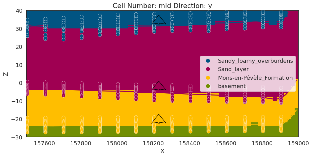

#Export geometry as vtk
_plot.export_to_vtk(geoModel, path='../Vtk/geoModel')

True

#export voxels as xyz
print(sol.lith_block.shape,sol.grid.values.shape)

(196875,) (196875, 3)

lithReshaped = sol.lith_block.reshape(sol.lith_block.shape[0],1)
lithReshaped

array([[4.        ],
       [4.        ],
       [4.        ],
       ...,
       [1.99742458],
       [1.        ],
       [1.        ]])

xyzLito = np.append(sol.grid.values,lithReshaped,axis=1)
xyzLito[:5]

array([[ 1.57510000e+05,  1.77010000e+05, -2.90000000e+01,
         4.00000000e+00],
       [ 1.57510000e+05,  1.77010000e+05, -2.70000000e+01,
         4.00000000e+00],
       [ 1.57510000e+05,  1.77010000e+05, -2.50000000e+01,
         4.00000000e+00],
       [ 1.57510000e+05,  1.77010000e+05, -2.30000000e+01,
         3.89641619e+00],
       [ 1.57510000e+05,  1.77010000e+05, -2.10000000e+01,
         3.00000000e+00]])

np.save('../Txt/output/xyzLito',xyzLito)

Blog

Geological modeling of sedimentary layers from geospatial rasters with Python and Gempy - Tutorial

Tutorial

Input data

Code

Geological data preparation

Geological modeling

Hatari Labs

Coming events: