Geospatial crop counting from drone orthophotos with Python, Scikit Learn and Scikit Image
/
Orthophoto from drones provide us aerial imagery with spatial resolution in the scale of centimeters. With this high definition and cheap orthophotos we can interpret, analyze and quantify objects on a horizontal distribution by means of machine learning libraries for image recognition and cluster analysis. We have done an applied example of plant recognition and counting from a drone orthophoto with Python and the machine learning libraries Scikit Learn and Scikit Image. The whole process is geospatial, as it works with raster and shapefiles and results are finally displayed on QGIS.
Tutorial
There is a previous tutorial for decreasing the resolution of a drone orthophoto on this link.
Input data
You can download the input data from this link.
Coding
This is the complete Python code for the tutorial:
#import required libraries
%matplotlib inline
import matplotlib.pyplot as plt
import geopandas as gpd
import rasterio
from rasterio.plot import show
from skimage.feature import match_template
import numpy as np
from PIL import Image
C:\Users\GIDA2\Anaconda3\lib\site-packages\geopandas\_compat.py:88: UserWarning: The Shapely GEOS version (3.4.3-CAPI-1.8.3 r4285) is incompatible with the GEOS version PyGEOS was compiled with (3.8.1-CAPI-1.13.3). Conversions between both will be slow.
shapely_geos_version, geos_capi_version_string#open point shapefile
pointData = gpd.read_file('Shp/pointData.shp')
print('CRS of Point Data: ' + str(pointData.crs))
#open raster file
palmRaster = rasterio.open('Rst/palmaOrthoTotal_14cm.tif')
print('CRS of Raster Data: ' + str(palmRaster.crs))
print('Number of Raster Bands: ' + str(palmRaster.count))
print('Interpretation of Raster Bands: ' + str(palmRaster.colorinterp))CRS of Point Data: epsg:4326
CRS of Raster Data: EPSG:4326
Number of Raster Bands: 4
Interpretation of Raster Bands: (<ColorInterp.red: 3>, <ColorInterp.green: 4>, <ColorInterp.blue: 5>, <ColorInterp.alpha: 6>)#show point and raster on a matplotlib plot
fig, ax = plt.subplots(figsize=(18,18))
pointData.plot(ax=ax, color='orangered', markersize=100)
show(palmRaster, ax=ax)C:\Users\GIDA2\Anaconda3\lib\site-packages\rasterio\plot.py:109: NodataShadowWarning: The dataset's nodata attribute is shadowing the alpha band. All masks will be determined by the nodata attribute
arr = source.read(rgb_indexes, masked=True)
<matplotlib.axes._subplots.AxesSubplot at 0x1ccb236e6c8>
#selected band: green
greenBand = palmRaster.read(2)
#extract point value from raster
surveyRowCol = []
for index, values in pointData.iterrows():
x = values['geometry'].xy[0][0]
y = values['geometry'].xy[1][0]
row, col = palmRaster.index(x,y)
print("Point N°:%d corresponds to row, col: %d, %d"%(index,row,col))
surveyRowCol.append([row,col])Point N°:0 corresponds to row, col: 848, 1162
Point N°:1 corresponds to row, col: 875, 1263
Point N°:2 corresponds to row, col: 689, 471
Point N°:3 corresponds to row, col: 1693, 1246
Point N°:4 corresponds to row, col: 1940, 1408
Point N°:5 corresponds to row, col: 1864, 1727
Point N°:6 corresponds to row, col: 1368, 1796
Point N°:7 corresponds to row, col: 1168, 1748
Point N°:8 corresponds to row, col: 979, 1279
Point N°:9 corresponds to row, col: 1108, 1407
Point N°:10 corresponds to row, col: 1147, 586
Point N°:11 corresponds to row, col: 473, 494
Point N°:12 corresponds to row, col: 1062, 667
Point N°:13 corresponds to row, col: 1136, 808# number of template images
print('Number of template images: %d'%len(surveyRowCol))
# define ratio of analysis
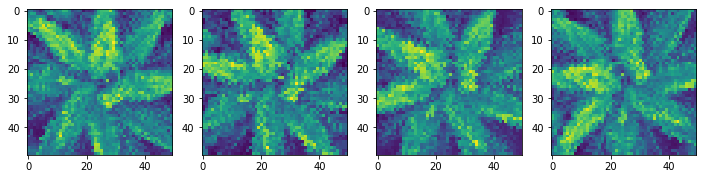
radio = 25Number of template images: 14#show all the points of interest, please be careful to have a complete image, otherwise the model wont run
fig, ax = plt.subplots(1, len(surveyRowCol),figsize=(20,5))
for index, item in enumerate(surveyRowCol):
row = item[0]
col = item[1]
ax[index].imshow(greenBand)
ax[index].plot(col,row,color='red', linestyle='dashed', marker='+',
markerfacecolor='blue', markersize=8)
ax[index].set_xlim(col-radio,col+radio)
ax[index].set_ylim(row-radio,row+radio)
ax[index].axis('off')
ax[index].set_title(index)
# Match the image to the template

listaresultados = []

templateBandList = []
for rowCol in surveyRowCol:
    imageList = []
    row = rowCol[0]
    col = rowCol[1]
    #append original band
    imageList.append(greenBand[row-radio:row+radio, col-radio:col+radio])
    #append rotated images
    templateBandToRotate = greenBand[row-2*radio:row+2*radio, col-2*radio:col+2*radio]
    rotationList = [i*30 for i in range(1,4)]
    for rotation in rotationList:
        rotatedRaw = Image.fromarray(templateBandToRotate)
        rotatedImage = rotatedRaw.rotate(rotation)
        imageList.append(np.asarray(rotatedImage)[radio:-radio,radio:-radio])
    #plot original and rotated images
    fig, ax = plt.subplots(1, len(imageList),figsize=(12,12))
    for index, item in enumerate(imageList):
        ax[index].imshow(imageList[index])
    #add images to total list
    templateBandList+=imageList


# match the template image to the orthophoto
matchXYList = []
for index, templateband in enumerate(templateBandList):
    if index%10 == 0:
        print('Match template ongoing for figure Nº %d'%index)
    matchTemplate = match_template(greenBand, templateband, pad_input=True)
    matchTemplateFiltered = np.where(matchTemplate>np.quantile(matchTemplate,0.9996))
    for item in zip(matchTemplateFiltered[0],matchTemplateFiltered[1]):
        x, y = palmRaster.xy(item[0], item[1])
        matchXYList.append([x,y])
Match template ongoing for figure Nº 0
Match template ongoing for figure Nº 10
Match template ongoing for figure Nº 20
Match template ongoing for figure Nº 30
Match template ongoing for figure Nº 40
Match template ongoing for figure Nº 50# plot interpreted points over the image
fig, ax = plt.subplots(figsize=(20, 20))
matchXYArray = np.array(matchXYList)
ax.scatter(matchXYArray[:,0],matchXYArray[:,1], marker='o',c='orangered', s=100, alpha=0.25)
show(palmRaster, ax=ax)<matplotlib.axes._subplots.AxesSubplot at 0x1ccba1d7408>
# cluster analysis
from sklearn.cluster import Birch
brc = Birch(branching_factor=10000, n_clusters=None, threshold=2e-5, compute_labels=True)
brc.fit(matchXYArray)
birchPoint = brc.subcluster_centers_
birchPoint
array([[-84.20038278, 9.48201204],
[-84.20064248, 9.48201099],
[-84.20022459, 9.48195993],
...,
[-84.20154469, 9.4803915 ],
[-84.20115389, 9.47998263],
[-84.20024387, 9.47971317]])# plot clustered points
fig = plt.figure(figsize=(20, 20))
ax = fig.add_subplot(111)
ax.scatter(birchPoint[:,[0]],birchPoint[:,[1]], marker='o',color='orangered',s=100)
show(palmRaster, ax=ax)
plt.show()