
Sensibility analysis of transient pumping test with MODFLOW-6, Flopy and SALib - Tutorial
/
Sensitivity analysis is referred to the uncertainty analysis in model results from the uncertainties on the model inputs (or something close to this definition). We usually perform this analysis on observation points (point that we know) with certain predefined ranges over the hydraulic parameters.
Python is an object oriented programming language and everything can be treated as an object like a MODFLOW-6 model. Having a pumping test model as an object allows us to use powerful Python libraries as SALib to perform sensibility analysis.
This tutorial covers the whole procedure to perform a sensitivity analysis over a 72 hour pumping test plus recovery on the hydraulic response in an observation piezometer located at 11 meters from the well. the Since the study case it’s a transient model the sensitivities will vary over time and stage of pumping/recovery.
Tutorial
Code
#import required packages
import os
from workingTools import paramModel
import pandas as pd
import numpy as np
import seaborn as sns
import matplotlib.pyplot as plt
#model parameters
simName = "mfsim.nam"
simWs = "../Model/pumpingTest/"
exeName = "../Bin/mf6.exe"
destDir = "../workingModel"#open model
parSim = paramModel(simName=simName,
simWs=simWs,
exeName=exeName,
destDir=destDir)parSim.loadSimulation()Check for files in 'C:\Users\saulm\Documents\webinarSensitivityAnalisysPumpingTestFlopySALib_v1\workingModel'.
Deleted file: C:\Users\saulm\Documents\webinarSensitivityAnalisysPumpingTestFlopySALib_v1\workingModel\mfsim.lst
Deleted file:
...
All files in 'C:\Users\saulm\Documents\webinarSensitivityAnalisysPumpingTestFlopySALib_v1\workingModel' have been deleted.
loading simulation...
loading simulation name file...
loading tdis package...
loading model gwf6...
loading package dis...
loading package npf...
loading package ic...
loading package sto...
loading package ghb...
loading package wel...
loading package oc...
loading package obs...
loading solution package pumpingtest...
Models in simulation: ['pumpingtest']#change place to store model
parSim.changeSimPath()#load model inside simulaiton
gwf = parSim.loadModel('pumpingTest')Package list: ['DIS', 'NPF', 'IC', 'STO', 'GHB_0', 'WEL_0', 'OC', 'OBS_0']#values of k and k33
parSim.uniqueValues('NPF','k')
parSim.uniqueValues('NPF','k33')
#values of sto
parSim.uniqueValues('STO','sy')
parSim.uniqueValues('STO','ss')k unique values: [1.e-06 1.e-05 3.e-05 1.e-03]
k33 unique values: [1.e-07 1.e-06 3.e-06 1.e-04]
sy unique values: [0.02]
ss unique values: [0.0001]#def runModelForParams(kLay4Org,kLay4,ss):
def runModelForParams(kLay2Org,kLay2,kLay3Org,kLay3,kLay4Org,kLay4,ss,anisotrophy):
simName = "mfsim.nam"
simWs = "../Model/pumpingTest/"
exeName = "../Bin/mf6.exe"
destDir = "../workingModel"
parSim = paramModel(simName=simName,
simWs=simWs,
exeName=exeName,
destDir=destDir)
parSim.loadSimulation()
parSim.changeSimPath()
gwf = parSim.loadModel('pumpingTest')
npf = gwf.get_package('NPF')
kArray = np.copy(npf.k.array)
kArray[kArray == kLay2Org] = kLay2
kArray[kArray == kLay3Org] = kLay3
kArray[kArray == kLay4Org] = kLay4
# npf.k = kArray
npf.k33 = kArray/anisotrophy
sto = gwf.get_package('STO')
ssArray = np.copy(sto.ss.array)
ssArray = np.ones(ssArray.shape)*ss
# syArray = np.copy(sto.sy.array)
# syArray = np.ones(syArray.shape)*sy
sto.ss = ssArray
# sto.sy = syArray
parSim.sim.write_simulation(silent=True)
parSim.sim.run_simulation(silent=True)
obs = gwf.get_package('OBS')
obsFile = list(obs.continuous.data.keys())[0]
piezoDf = pd.read_csv(os.path.join(destDir,obsFile))
piezoArray = piezoDf['11J025'].values
return piezoArray# run the model function for certain parameters
piezoData = runModelForParams(kLay2Org = 1.e-5,
kLay2 = 2.e-5,
kLay3Org = 1.e-6,
kLay3 = 2.e-6,
kLay4Org = 3.e-5,
kLay4 = 4.e-5,
ss = 0.01,
anisotrophy = 12)
piezoDataCheck for files in 'C:\Users\saulm\Documents\webinarSensitivityAnalisysPumpingTestFlopySALib_v1\workingModel'.
All files in 'C:\Users\saulm\Documents\webinarSensitivityAnalisysPumpingTestFlopySALib_v1\workingModel' have been deleted.
loading simulation...
loading simulation name file...
loading tdis package...
loading model gwf6...
loading package dis...
loading package npf...
loading package ic...
loading package sto...
loading package ghb...
loading package wel...
loading package oc...
loading package obs...
loading solution package pumpingtest...
Models in simulation: ['pumpingtest']
Package list: ['DIS', 'NPF', 'IC', 'STO', 'GHB_0', 'WEL_0', 'OC', 'OBS_0']
array([36.06409234, 36.06405133, 36.06190622, 36.03339522, 35.8784959 ,
35.42731328, 34.57162642, 33.34713003, 31.87685404, 31.51837171,
30.95411132, 30.15079804, 29.75989431, 29.42619987, 29.13623893,
29.13287467, 29.12823318, 29.14326545, 29.27157487, 29.67097245,
30.42815125, 31.4727085 , 32.63476689, 33.17286159, 33.56929893,
33.87399851, 34.11589212, 34.31282313, 34.47639416])#numbre of records
piezoData.shape[0]29Perform sensibility analysis with SALib
import SALib.sample.sobol as sobolSample
from SALib.analyze import sobol
from SALib.test_functions import Ishigami
# Define the model inputs
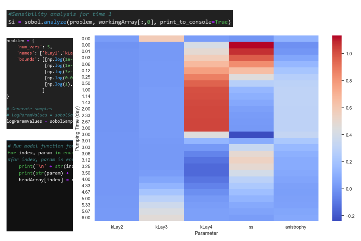
problem = {
'num_vars': 5,
'names': ['kLay2','kLay3','kLay4','ss','anistrophy'],
'bounds': [[np.log(1e-6),np.log(1e-4)], #1.e-5
[np.log(1e-7),np.log(1e-5)], #1.e-6
[np.log(3e-6),np.log(3e-3)], #3.e-5
[np.log(0.00001),np.log(0.001)], #0.0001
[np.log(1),np.log(100)], #10
]
}
# Generate samples
logParamValues = sobolSample.sample(problem,16)
# Print number of groups and paramenters
print(logParamValues.shape)(192, 5)# Create empty array
headArray = np.zeros([logParamValues.shape[0],piezoData.shape[0]])
print(headArray.shape)(192, 29)# Run model function for every group of params
for index, param in enumerate(logParamValues):
#for index, param in enumerate(logParamValues[:10]):
print('\n' + str(index) + '\n')
print(str(param) + '\n')
headArray[index] = runModelForParams(kLay2Org = 1.e-5,
kLay2 = np.e**param[0],
kLay3Org = 1.e-6,
kLay3 = np.e**param[1],
kLay4Org = 3.e-5,
kLay4 = np.e** param[2],
ss = np.e**param[3],
anisotrophy = np.e**param[4])# Review result for time 1
# headArray = headArray[:10]
# headArrayMod = np.repeat(headArray[:10], 13, axis=0)
# headArrayMod = headArrayMod[:-1]
# headArrayMod.shapeheadArray# saveResults
np.save('../Txt/headArray.npy', headArray)
# np.save('../Txt/headArray.npy', headArrayMod)#loadResults
#workingArray = np.load('../Txt/headArray.npy')
workingArray = np.load('../Txt/headArrayBackup.npy')
workingArray.shape(192, 29)workingArray[:,18]array([33.03916432, 33.03915915, 33.05577217, 32.83254251, 33.69856109,
33.13917427, 33.62722586, 33.61065915, 33.79878946, 32.94971915,
33.53825786, 33.62605225, 34.18646187, 34.26730819, 34.07744032,
....workingArray[:,0].shape(192,)#Sensibility analysis for time 1
Si = sobol.analyze(problem, workingArray[:,0], print_to_console=True)ST ST_conf
kLay2 0.049171 0.085312
kLay3 0.477092 0.537714
kLay4 0.033920 0.131855
ss 0.000000 0.000000
anistrophy 0.402161 0.646762
S1 S1_conf
kLay2 0.030444 0.109832
kLay3 0.582632 0.428772
kLay4 0.024199 0.140710
ss 0.000000 0.000000
anistrophy 0.117297 0.238550
S2 S2_conf
(kLay2, kLay3) -2.078223e-01 3.737154e-01
(kLay2, kLay4) -7.634057e-02 1.407600e-01
(kLay2, ss) -6.552616e-02 1.571205e-01
(kLay2, anistrophy) -4.892194e-02 1.641585e-01
(kLay3, kLay4) -5.215442e-01 7.039154e-01
(kLay3, ss) -5.303412e-01 6.482610e-01
(kLay3, anistrophy) -5.561421e-01 6.102043e-01
(kLay4, ss) -1.746956e-02 1.312337e-01
(kLay4, anistrophy) -1.567016e-02 1.222106e-01
(ss, anistrophy) -1.387779e-17 5.336056e-17# Print the first-order sensitivity indices
print(problem['names'])
print(Si['S1'])['kLay2', 'kLay3', 'kLay4', 'ss', 'anistrophy']
[0.03044394 0.58263189 0.02419889 0. 0.11729659]### Sensibility analysis for all piezometerssensArray = np.zeros([piezoData.shape[0],problem['num_vars']])
for piezo in range(piezoData.shape[0]):
Si = sobol.analyze(problem, workingArray[:,piezo])
sensArray[piezo] = Si['S1']
sensArrayarray([[ 3.04439433e-02, 5.82631887e-01, 2.41988869e-02,
0.00000000e+00, 1.17296593e-01],
[-5.81952351e-03, 1.52109190e-02, 4.13381511e-01,
1.13354539e+00, -1.57075509e-02],
[-3.66126750e-03, 1.32241987e-02, 4.89127346e-01,
1.07379966e+00, 6.66554747e-03].....#get times as days
timeList = ['%.2f'%(tim/86400) for tim in gwf.modeltime.totim]
timeList[:5]['0.00', '0.00', '0.01', '0.03', '0.06']#plot sensibilities as heatmap
np.random.seed(0)
sns.set()
sns.dark_palette("palegreen", as_cmap=True)
fig = plt.figure(figsize=(12,8))
ax = sns.heatmap(sensArray,
xticklabels=problem['names'], yticklabels=timeList,
cmap="coolwarm")
ax.grid(alpha=0.5)
ax.set_ylabel('Pumping Time (day)')
ax.set_xlabel('Parameter')Text(0.5, 55.249999999999986, 'Parameter')
Input files
You can download the input files from this link.
https://owncloud.hatarilabs.com/s/inyE6XC9heQtgIr
Password to download data: Hatarilabs