How to delineate crop rows with machine learning using Python and Scikit Learn - Tutorial

Drone imagery shows us features on the surface with high precision and machine learning tools allows us to understand and get information from those images. We present a tutorial in Python together with Scikit Learn and geospatial libraries that delineates crop rows on a corn field and provides results as a vector spatial file. 

The tutorial can be done with Anaconda with all the required libraries installed or with the Hakuchik image on Docker. To run Hakuchik you need Docker installed and then run this line on Bash / Powershell:

docker run -it --name hakuchik -p 8888:8888 -p 6543:5432 hatarilabs/hakuchik:a2d1cb82a605

This is the Github repository of the tutorial:

https://github.com/SaulMontoya/howToDetectCropRowswithPythonScikitImage

Code

Import required packages

#python and matplotlib libraries
import numpy as np
import math 
import matplotlib.pyplot as plt
from matplotlib import cm, gridspec

#geospatial libraries
import rasterio
import fiona
import geopandas as gpd

#machine learning libraries
#!pip install scikit-image
from skimage import feature
from skimage.transform import hough_line, hough_line_peaks

Import raster and read band

imgRaster = rasterio.open('../Rst/corn.tif')
im = imgRaster.read(1)
fig = plt.figure(figsize=(12,8))
plt.imshow(im)
plt.show()

Canny filter

# Compute the Canny filter for two values of sigma
edges1 = feature.canny(im)
edges2 = feature.canny(im, sigma=3)

# display results
fig, (ax1, ax2, ax3) = plt.subplots(nrows=1, ncols=3, figsize=(18, 6),
                                    sharex=True, sharey=True)

ax1.imshow(im, cmap=plt.cm.gray)
ax1.axis('off')
ax1.set_title('noisy image', fontsize=20)

ax2.imshow(edges1, cmap=plt.cm.gray)
ax2.axis('off')
ax2.set_title(r'Canny filter, $\sigma=1$', fontsize=20)

ax3.imshow(edges2, cmap=plt.cm.gray)
ax3.axis('off')
ax3.set_title(r'Canny filter, $\sigma=3$', fontsize=20)

fig.tight_layout()

plt.show()

Hough line transform

selImage = edges2

# Classic straight-line Hough transform
# Set a precision of 2 degree.

precision = 2

tested_angles = np.linspace(-np.pi / 2, np.pi / 2, int(180 / precision), endpoint=False)
h, theta, d = hough_line(selImage, theta=tested_angles)

# Generating figure 1
fig = plt.figure(figsize=(18, 16))
gs = gridspec.GridSpec(2,2)

ax0 = plt.subplot(gs[0,0])
ax0.imshow(selImage, cmap=cm.YlGnBu)
ax0.set_title('Input image')
ax0.set_axis_off()

ax1 = plt.subplot(gs[:,1])
angle_step = 0.5 * np.diff(theta).mean()
d_step = 0.5 * np.diff(d).mean()
bounds = [np.rad2deg(theta[0] - angle_step),
          np.rad2deg(theta[-1] + angle_step),
          d[-1] + d_step, d[0] - d_step]
ax1.imshow(np.log(1 + h), extent=bounds, cmap=cm.YlGn, aspect=1 / 1.5)
ax1.set_title('Hough transform')
ax1.set_xlabel('Angles (degrees)')
ax1.set_ylabel('Distance (pixels)')
ax1.axis('image')
ax1.set_aspect(.2)

ax2 = plt.subplot(gs[1,0])
ax2.imshow(selImage, cmap=cm.YlGn)
ax2.set_ylim((selImage.shape[0], 0))
ax2.set_xlim((0,selImage.shape[1]))
ax2.set_axis_off()
ax2.set_title('Detected lines')

for _, angle, dist in zip(*hough_line_peaks(h, theta, d)):
    (x0, y0) = dist * np.array([np.cos(angle), np.sin(angle)])
    ax2.axline((x0, y0), slope=np.tan(angle + np.pi/2))

plt.tight_layout()
plt.show()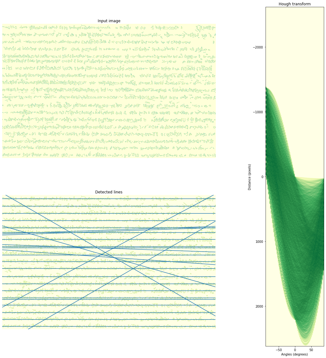

Transform results to geospatial information

#define representative length of interpreted lines in pixels
#selDiag = int(np.sqrt(selImage.shape[0]**2+selImage.shape[1]**2))
selDiag = selImage.shape[1]
progRange = range(selDiag)

totalLines = []
angleList = []
for _, angle, dist in zip(*hough_line_peaks(h, theta, d)):
    (x0, y0) = dist * np.array([np.cos(angle), np.sin(angle)])
    if angle in [np.pi/2, -np.pi/2]:
        cols = [prog for prog in progRange]
        rows = [y0 for prog in progRange]
    elif angle == 0:
        cols = [x0 for prog in progRange]
        rows = [prog for prog in progRange]
    else:
        c0 = y0 + x0 / np.tan(angle)
        cols = [prog for prog in progRange]
        rows = [col*np.tan(angle + np.pi/2) + c0 for col in cols]

    partialLine = []
    for col, row in zip(cols, rows):
        partialLine.append(imgRaster.xy(row,col))
    totalLines.append(partialLine)
    if math.degrees(angle+np.pi/2) > 90:
        angleList.append(180 - math.degrees(angle+np.pi/2))
    else:
        angleList.append(math.degrees(angle+np.pi/2))

#show on sample of the points and lines
print(totalLines[0][:5])
print(angleList)

[(490717.0137014835, 5262376.552876524), (490717.02391147637, 5262376.552876524), (490717.03412146925, 5262376.552876524), (490717.0443314621, 5262376.552876524), (490717.054541455, 5262376.552876524)]
[0.0, 0.0, 0.0, 0.0, 0.0, 0.0, 0.0, 0.0, 0.0, 0.0, 0.0, 0.0, 0.0, 0.0, 0.0, 0.0, 0.0, 0.0, 0.0, 0.0, 0.0, 2.0, 28.0, 15.999999999999996, 2.0, 4.000000000000005, 2.0000000000000027, 29.999999999999993, 30.0]

Save the resulting lines to shapefile

#define schema
schema = {
    'properties':{'angle':'float:16'},
    'geometry':'LineString'
}

#out shapefile
outShp = fiona.open('../Shp/croprows.shp',mode='w',driver='ESRI Shapefile',schema=schema,crs=imgRaster.crs)
for index, line in enumerate(totalLines):
    feature = {
        'geometry':{'type':'LineString','coordinates':line},
        'properties':{'angle':angleList[index]}
         }
    outShp.write(feature)
outShp.close()

#out geojson
outJson = fiona.open('../Shp/croprows.geojson',mode='w',driver='GeoJSON',schema=schema,crs=imgRaster.crs)
for index, line in enumerate(totalLines):
    feature = {
        'geometry':{'type':'LineString','coordinates':line},
        'properties':{'angle':angleList[index]}
         }
    outJson.write(feature)
outJson.close()

Representation of the interpreted crop rows

df = gpd.read_file('../Shp/croprows.shp')
fig, ax = plt.subplots(figsize=(12,8))
lineShow = df.plot(column='angle', cmap='RdBu', ax=ax)
plt.show()