Finite difference method as well as any other discretization method allows the conceptualization of a geological media into cells or other volumes. Geological models come in diverse formats in binary or text format and need to be “translated” to the cell extension of a groundwater model.

This tutorial has a applied example of the implementation of a 3D geological model from a neural network into a groundwater model with determined horizontal discretization and layer thickness. The tutorial covers all the steps for model construction and hydrogeological unit determination with scripts in Python with Flopy and other libraries. Comparisons of the original and translated geological model were done as Matplotlib plots and Vtk files in Paraview.

Video

Scripts

This is the main Python script of the tutorial:

import os
import flopy
import numpy as np
import pandas as pd
import matplotlib.pyplot as plt
from flopy.utils.reference import SpatialReference
from scipy.interpolate import griddata
from shapely.geometry import Polygon

flopy is installed in /home/wk-gida1/.local/lib/python3.7/site-packages/flopy

xMin = 540000
xMax = 560000
yMin = 4820000
yMax = 4840000
aoiGeom = Polygon(((xMin,yMin),(xMax,yMin),(xMax,yMax),(xMin,yMax),(xMin,yMin)))

cellH = 250

vertexCols = np.arange(xMin,xMax+1,cellH)
vertexRows = np.arange(yMax,yMin-1,-cellH)
cellCols = (vertexCols[1:]+vertexCols[:-1])/2
cellRows = (vertexRows[1:]+vertexRows[:-1])/2 
nCols = cellCols.shape[0]
nRows = cellRows.shape[0]

Creation of a model topo

# Open well location:
wellLoc = pd.read_csv("../inputData/TV-HFM_Wells_1Location_Wgs11N.csv",index_col=0)
wellLoc.head()

	Easting	Northing	Altitude_ft	EastingUTM	NorthingUTM	Elevation_m
Bore
A. Isaac	2333140.95	1372225.65	3204.0	575546.628834	4.820355e+06	976.57920
A. Woodbridge	2321747.00	1360096.95	2967.2	564600.366582	4.807827e+06	904.40256
A.D. Watkins	2315440.16	1342141.86	3168.3	558944.843404	4.789664e+06	965.69784
A.L. Clark; 1	2276526.30	1364860.74	2279.1	519259.006159	4.810959e+06	694.66968
A.L. Clark; 2	2342620.87	1362980.46	3848.6	585351.150270	4.811460e+06	1173.05328

points = wellLoc[['EastingUTM','NorthingUTM']].values
values = wellLoc['Elevation_m'].values
grid_x = np.tile(cellCols,(nRows,1))
grid_y = np.tile(cellRows,(nCols,1)).T
mtop = griddata(points, values, (grid_x, grid_y), method='linear')
print(mtop[:5,:5])
print(mtop.max())

[[769.26668708 769.93247791 770.59826874 771.26405958 771.92985041]
 [767.33963938 768.00543022 768.67122105 769.33701188 770.00280272]
 [765.41259169 766.07838252 766.74417336 767.40996419 768.07575502]
 [763.70469671 764.15133483 764.81712566 765.4829165  766.14870733]
 [762.36605826 762.22428714 762.89007797 763.55586881 764.22165964]]
930.0534171904137

plt.imshow(mtop)

<matplotlib.image.AxesImage at 0x7f3fe0c3ddd0>

Modflow model object and DIS package

modelname='Model1'
model_ws= '../Model'
mf = flopy.modflow.Modflow(modelname, exe_name="../../../Solvers/mfnwt", version="mfnwt",model_ws=model_ws)

#Definition of MODFLOW NWT Solver
nwt = flopy.modflow.ModflowNwt(mf ,maxiterout=250,linmeth=2,headtol=0.01,Continue=True)

# setting up the vertical discretization and model bottom elevation
nLays = 5
AcuifInf_Bottom = 500

zbot = np.zeros((nLays,nRows,nCols))
zbot[0,:,:] = AcuifInf_Bottom + (0.88 * (mtop - AcuifInf_Bottom))
zbot[1,:,:] = AcuifInf_Bottom + (0.76 * (mtop - AcuifInf_Bottom))
zbot[2,:,:] = AcuifInf_Bottom + (0.6 * (mtop - AcuifInf_Bottom))
zbot[3,:,:] = AcuifInf_Bottom + (0.4 * (mtop - AcuifInf_Bottom))
zbot[4,:,:] = AcuifInf_Bottom

# Dis package
dis = flopy.modflow.ModflowDis(mf, nlay=nLays,
                               nrow=nRows,ncol=nCols,
                               delr=cellH,delc=cellH,
                               top=mtop,botm=zbot,
                               itmuni=1.,nper=1,perlen=1,nstp=1,steady=True)

mf.modelgrid.set_coord_info(xoff=xMin, yoff=yMin, angrot=0,epsg=32611)

fig = plt.figure(figsize=(12,8))
ax = fig.add_subplot(1, 1, 1, aspect='equal')
modelmap = flopy.plot.PlotMapView(model=mf)
linecollection = modelmap.plot_grid(linewidth=0.5, color='royalblue')

fig = plt.figure(figsize=(20, 6))
ax = fig.add_subplot(1, 1, 1)
modelxsect = flopy.plot.PlotCrossSection(model=mf, line={'Column': 0})
linecollection = modelxsect.plot_grid()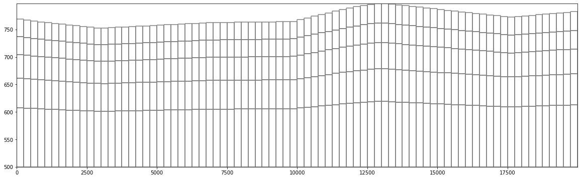

Apply the lithological model and UPW package

#open the 3D lithological model as x,y,z,lito list
zVerts = mf.modelgrid.zvertices
litoList = np.load("../processedData/litoListXYZL.npy")
print(litoList[:5])
print(litoList[-1])
print(litoList.shape)

#initialization of model hydraulic conductivity
hK = np.zeros([nLays,nRows,nCols])

[[5.4010e+05 4.8399e+06 8.2900e+02 3.0000e+00]
 [5.4030e+05 4.8399e+06 8.2900e+02 3.0000e+00]
 [5.4050e+05 4.8399e+06 8.2900e+02 3.0000e+00]
 [5.4070e+05 4.8399e+06 8.2900e+02 3.0000e+00]
 [5.4090e+05 4.8399e+06 8.2900e+02 3.0000e+00]]
[5.5990e+05 4.8201e+06 5.4900e+02 3.0000e+00]
(150000, 4)

import statistics, copy
i=0
for lay in range(nLays):
    for row in range(nRows):
        for col in range(nCols):
            cellXMin = vertexCols[col]
            cellXMax = vertexCols[col+1]
            cellYMin = vertexRows[row+1]
            cellYMax = vertexRows[row]
            cellZMin = zVerts[lay+1,row,col]
            cellZMax = zVerts[lay,row,col]

            litoAux = copy.copy(litoList)
            litoAux = litoAux[litoAux[:,0] >= cellXMin]
            litoAux = litoAux[litoAux[:,0] < cellXMax]
            litoAux = litoAux[litoAux[:,1] >= cellYMin]
            litoAux = litoAux[litoAux[:,1] < cellYMax]
            litoAux = litoAux[litoAux[:,2] >= cellZMin]
            litoAux = litoAux[litoAux[:,2] < cellZMax]


            litoValues = list(litoAux[:,3])

            if len(litoValues)>0:
                try:
                    litoMode = statistics.mode(litoValues)
                except statistics.StatisticsError:
                    litoMode = max(litoValues)            
            else:
                print("No values found %s"%str([lay,row,col]))
                litoMode = 1

            if i%5000==0:
                print(lay,row,col)
                print(litoValues)
                print(litoMode)
            i+=1

            hK[lay,row,col]=litoMode

0 0 0
[2.0, 2.0]
2.0
No values found [0, 0, 70]
No values found [0, 0, 71]
No values found [0, 0, 72]
No values found [0, 0, 73]
No values found [0, 0, 74]
No values found [0, 0, 75]
No values found [0, 0, 76]
No values found [0, 0, 77]
No values found [0, 0, 78]
No values found [0, 0, 79]
No values found [0, 1, 71]
No values found [0, 1, 72]
No values found [0, 1, 73]
No values found [0, 1, 74]
No values found [0, 1, 75]
No values found [0, 1, 76]
No values found [0, 1, 77]
No values found [0, 1, 78]
No values found [0, 1, 79]
No values found [0, 2, 72]
No values found [0, 2, 73]
No values found [0, 2, 74]
No values found [0, 2, 75]
No values found [0, 2, 76]
No values found [0, 2, 77]
No values found [0, 2, 78]
No values found [0, 2, 79]
No values found [0, 3, 73]
No values found [0, 3, 74]
No values found [0, 3, 75]
No values found [0, 3, 76]
No values found [0, 3, 77]
No values found [0, 3, 78]
No values found [0, 3, 79]
No values found [0, 4, 74]
No values found [0, 4, 75]
No values found [0, 4, 76]
No values found [0, 4, 77]
No values found [0, 4, 78]
No values found [0, 4, 79]
No values found [0, 5, 75]
No values found [0, 5, 76]
No values found [0, 5, 77]
No values found [0, 5, 78]
No values found [0, 5, 79]
No values found [0, 6, 76]
No values found [0, 6, 77]
No values found [0, 6, 78]
No values found [0, 6, 79]
No values found [0, 7, 77]
No values found [0, 7, 78]
No values found [0, 7, 79]
No values found [0, 8, 78]
No values found [0, 8, 79]
No values found [0, 9, 79]
0 62 40
[1.0, 1.0]
1.0
No values found [0, 76, 77]
No values found [0, 76, 78]
No values found [0, 76, 79]
No values found [0, 77, 73]
No values found [0, 77, 74]
No values found [0, 77, 75]
No values found [0, 77, 76]
No values found [0, 77, 77]
No values found [0, 77, 78]
No values found [0, 77, 79]
No values found [0, 78, 72]
No values found [0, 78, 73]
No values found [0, 78, 74]
No values found [0, 78, 75]
No values found [0, 78, 76]
No values found [0, 78, 77]
No values found [0, 78, 78]
No values found [0, 78, 79]
No values found [0, 79, 71]
No values found [0, 79, 72]
No values found [0, 79, 73]
No values found [0, 79, 74]
No values found [0, 79, 75]
No values found [0, 79, 76]
No values found [0, 79, 77]
No values found [0, 79, 78]
No values found [0, 79, 79]
1 45 0
[2.0, 2.0, 2.0, 2.0]
2.0
2 27 40
[1.0, 1.0]
1.0
3 10 0
[2.0, 2.0, 2.0]
2.0
3 72 40
[3.0, 3.0, 3.0, 3.0]
3.0
4 55 0
[3.0, 2.0, 2.0, 2.0]
2.0

# Definition of layer type, the first two layers are convertible
laytyp = [1,1,0,0,0]
upw = flopy.modflow.ModflowUpw(mf, laytyp = laytyp, hk=hK, vka=hK, ss=5e-06, sy=0.12) #vka= Kx,

fig = plt.figure(figsize=(20, 3))
ax = fig.add_subplot(1, 1, 1)
modelxsect = flopy.plot.PlotCrossSection(model=mf, line={'Row': 0})
linecollection = modelxsect.plot_grid()
modelxsect.plot_array(hK)

<matplotlib.collections.PatchCollection at 0x7f3fdfc97f50>

mf.write_input()

Input data

You can download the input files for this tutorial here.

Data source

Bartolino, J.R., 2019, Hydrogeologic framework of the Treasure Valley and surrounding area, Idaho and Oregon: U.S. Geological Survey Scientific Investigations Report 2019–5138, 31 p., https://doi.org/10.3133/sir20195138.

Bartolino, J.R., 2020, Hydrogeologic Framework of the Treasure Valley and Surrounding Area, Idaho and Oregon: U.S. Geological Survey data release, https://doi.org/10.5066/P9CAC0F6.