
3D Geological Models using Neural Networks with Python Scikit Learn and Vtk - Tutorial
/
Geoscientists need the best estimation of the geological environment to perform simulations or evaluations. Besides the geological background, building geological models also requires a whole set of mathematical methods as Bayesian networks, Cokrigging, SVM, Neural networks, Stochastic models to define which could be the rock type / property when information from drilling logs or geophysics is really scarce or uncertain.
We have done a tutorial in Python and recent and powerful libraries as Scikit Learn to create a geological model based on lithology from drillings on the Treasure Valley (Idaho, USA). The tutorial generates a point cloud of drillings lithologies that are transformed and scaled for the neural network. The selected neural network classifier is Multi-layer Perceptron classifier implemented on the Scikit Learn library as sklearn.neural_network.MLPClassifier. An analysis of the confusion from the neural network is performed. The tutorial also includes a georeferenced 3D visualization from well lithology and interpolated geology as Vtk format in Paraview.
Video
Scripts
This is the whole Python script used for the tutorial:
#import required libraries
%matplotlib inline
import os
import numpy as np
import pandas as pd
import matplotlib.pyplot as plt
import pyvista as pv
import vtk
Import well location and lithology
From the publicacion: https://pubs.usgs.gov/sir/2019/5138/sir20195138_v1.1.pdf The selected units would be:
- Coarse-grained fluvial and alluvial deposits
- Pliocene-Pleistocene and Miocene basalts
- Fine-grained lacustrine deposits
- Rhyolitic and granitic bedrock
wellLoc = pd.read_csv('../inputData/TV-HFM_Wells_1Location_Wgs11N.csv',index_col=0)
wellLoc.head()| Easting | Northing | Altitude_ft | EastingUTM | NorthingUTM | Elevation_m | |
|---|---|---|---|---|---|---|
| Bore | ||||||
| A. Isaac | 2333140.95 | 1372225.65 | 3204.0 | 575546.628834 | 4.820355e+06 | 976.57920 |
| A. Woodbridge | 2321747.00 | 1360096.95 | 2967.2 | 564600.366582 | 4.807827e+06 | 904.40256 |
| A.D. Watkins | 2315440.16 | 1342141.86 | 3168.3 | 558944.843404 | 4.789664e+06 | 965.69784 |
| A.L. Clark; 1 | 2276526.30 | 1364860.74 | 2279.1 | 519259.006159 | 4.810959e+06 | 694.66968 |
| A.L. Clark; 2 | 2342620.87 | 1362980.46 | 3848.6 | 585351.150270 | 4.811460e+06 | 1173.05328 |
wellLito = pd.read_csv('../inputData/TV-HFM_Wells_2Lithology_m_rcl_clip.csv',index_col=0)
wellLito.head()| Bore | Depth_top_L | Depth_bot_L | PrimaryLith | topLitoElev_m | botLitoElev_m | litoCode | hydrogeoCode | |
|---|---|---|---|---|---|---|---|---|
| 1309 | H. Raff | 0.0 | 1.0 | Soil | 770.44296 | 770.13816 | 0 | 1 |
| 1310 | H. Raff | 1.0 | 6.0 | Clay | 770.13816 | 768.61416 | 7 | 3 |
| 1311 | H. Raff | 6.0 | 12.0 | Gravel | 768.61416 | 766.78536 | 6 | 1 |
| 1312 | H. Raff | 12.0 | 18.0 | Clay | 766.78536 | 764.95656 | 7 | 3 |
| 1313 | H. Raff | 18.0 | 48.0 | Gravel | 764.95656 | 755.81256 | 6 | 1 |
Point cloud of lithologies
litoPoints = []

for index, values in wellLito.iterrows():
    wellX, wellY, wellZ = wellLoc.loc[values.Bore][["EastingUTM","NorthingUTM","Elevation_m"]]
    wellXY = [wellX, wellY]
    litoPoints.append(wellXY + [values.topLitoElev_m,values.hydrogeoCode])
    litoPoints.append(wellXY + [values.botLitoElev_m,values.hydrogeoCode])

    litoLength = values.topLitoElev_m - values.botLitoElev_m
    if litoLength < 1:
        midPoint = wellXY + [values.topLitoElev_m - litoLength/2,values.hydrogeoCode]
    else:
        npoints = int(litoLength)
        for point in range(1,npoints+1):
            disPoint = wellXY + [values.topLitoElev_m - litoLength*point/(npoints+1),values.hydrogeoCode]
            litoPoints.append(disPoint)
litoNp=np.array(litoPoints)
np.save('../outputData/litoNp',litoNp)
litoNp[:5]
array([[5.48261389e+05, 4.83802316e+06, 7.70442960e+02, 1.00000000e+00],
[5.48261389e+05, 4.83802316e+06, 7.70138160e+02, 1.00000000e+00],
[5.48261389e+05, 4.83802316e+06, 7.70138160e+02, 3.00000000e+00],
[5.48261389e+05, 4.83802316e+06, 7.68614160e+02, 3.00000000e+00],
[5.48261389e+05, 4.83802316e+06, 7.69376160e+02, 3.00000000e+00]])Coordinate transformation and Neural Network Classifier setup
from sklearn.neural_network import MLPClassifier
from sklearn.metrics import confusion_matrix
from sklearn import preprocessing
litoX, litoY, litoZ = litoNp[:,0], litoNp[:,1], litoNp[:,2]
litoMean = litoNp[:,:3].mean(axis=0)
litoTrans = litoNp[:,:3]-litoMean
litoTrans[:5]
#setting up scaler
scaler = preprocessing.StandardScaler().fit(litoTrans)
litoScale = scaler.transform(litoTrans)
#check scaler
print(litoScale.mean(axis=0))
print(litoScale.std(axis=0))[ 2.85924590e-14 -1.10313442e-15 3.89483608e-20]
[1. 1. 1.]#run classifier
X = litoScale
Y = litoNp[:,3]
clf = MLPClassifier(activation='tanh',solver='lbfgs',hidden_layer_sizes=(15,15,15), max_iter=2000)
clf.fit(X,Y)C:\Users\Gida\Anaconda3\lib\site-packages\sklearn\neural_network\_multilayer_perceptron.py:470: ConvergenceWarning: lbfgs failed to converge (status=1):
STOP: TOTAL NO. of ITERATIONS REACHED LIMIT.
Increase the number of iterations (max_iter) or scale the data as shown in:
https://scikit-learn.org/stable/modules/preprocessing.html
self.n_iter_ = _check_optimize_result("lbfgs", opt_res, self.max_iter)
MLPClassifier(activation='tanh', alpha=0.0001, batch_size='auto', beta_1=0.9,
beta_2=0.999, early_stopping=False, epsilon=1e-08,
hidden_layer_sizes=(15, 15, 15), learning_rate='constant',
learning_rate_init=0.001, max_fun=15000, max_iter=2000,
momentum=0.9, n_iter_no_change=10, nesterovs_momentum=True,
power_t=0.5, random_state=None, shuffle=True, solver='lbfgs',
tol=0.0001, validation_fraction=0.1, verbose=False,
warm_start=False)Determination of confusion matrix
numberSamples = litoNp.shape[0]
expected=litoNp[:,3]
predicted = []
for i in range(numberSamples):
    predicted.append(clf.predict([litoScale[i]]))
results = confusion_matrix(expected,predicted)
print(results)
[[1370 128 377 0]
[ 67 2176 10 0]
[ 274 33 1114 0]
[ 1 0 0 151]]Area of study and output grid refinement
xMin = 540000
xMax = 560000
yMin = 4820000
yMax = 4840000
zMax = int(wellLito.topLitoElev_m.max())
zMin = zMax - 300
cellH = 200
cellV = 20Determination of the lithology matrix
vertexCols = np.arange(xMin,xMax+1,cellH)
vertexRows = np.arange(yMax,yMin-1,-cellH)
vertexLays = np.arange(zMax,zMin-1,-cellV)
cellCols = (vertexCols[1:]+vertexCols[:-1])/2
cellRows = (vertexRows[1:]+vertexRows[:-1])/2
cellLays = (vertexLays[1:]+vertexLays[:-1])/2
nCols = cellCols.shape[0]
nRows = cellCols.shape[0]
nLays = cellLays.shape[0]
i=0
litoMatrix=np.zeros([nLays,nRows,nCols])
for lay in range(nLays):
for row in range(nRows):
for col in range(nCols):
cellXYZ = [cellCols[col],cellRows[row],cellLays[lay]]
cellTrans = cellXYZ - litoMean
cellNorm = scaler.transform([cellTrans])
litoMatrix[lay,row,col] = clf.predict(cellNorm)
if i%30000==0:
print("Processing %s cells"%i)
print(cellTrans)
print(cellNorm)
print(litoMatrix[lay,row,col])
i+=1Processing 0 cells
[-8553.96427073 8028.26104284 356.7050941 ]
[[-1.41791371 2.42904321 1.11476509]]
3.0
Processing 30000 cells
[-8553.96427073 8028.26104284 296.7050941 ]
[[-1.41791371 2.42904321 0.92725472]]
3.0
Processing 60000 cells
[-8553.96427073 8028.26104284 236.7050941 ]
[[-1.41791371 2.42904321 0.73974434]]
3.0
Processing 90000 cells
[-8553.96427073 8028.26104284 176.7050941 ]
[[-1.41791371 2.42904321 0.55223397]]
2.0
Processing 120000 cells
[-8553.96427073 8028.26104284 116.7050941 ]
[[-1.41791371 2.42904321 0.3647236 ]]
2.0plt.imshow(litoMatrix[0])<matplotlib.image.AxesImage at 0x14fb8688860>
plt.imshow(litoMatrix[:,60])

<matplotlib.image.AxesImage at 0x14fb871d390>
np.save('../outputData/litoMatrix',litoMatrix)

#matrix modification for Vtk representation
litoMatrixMod = litoMatrix[:,:,::-1]
np.save('../outputData/litoMatrixMod',litoMatrixMod)
plt.imshow(litoMatrixMod[0])

<matplotlib.image.AxesImage at 0x14fb87825f8>
Generation of regular grid VTK
import pyvista
import vtk

# Create empty grid
grid = pyvista.RectilinearGrid()

# Initialize from a vtk.vtkRectilinearGrid object
vtkgrid = vtk.vtkRectilinearGrid()
grid = pyvista.RectilinearGrid(vtkgrid)
grid = pyvista.RectilinearGrid(vertexCols,vertexRows,vertexLays)

litoFlat = list(litoMatrixMod.flatten(order="K"))[::-1]
grid.cell_arrays["hydrogeoCode"] = np.array(litoFlat)
grid.save('../outputData/hydrogeologicalUnit.vtk')
Input data
You can download the input data for this tutorial from the following link.
Data source
Bartolino, J.R., 2019, Hydrogeologic framework of the Treasure Valley and surrounding area, Idaho and Oregon: U.S. Geological Survey Scientific Investigations Report 2019–5138, 31 p., https://doi.org/10.3133/sir20195138.
Bartolino, J.R., 2020, Hydrogeologic Framework of the Treasure Valley and Surrounding Area, Idaho and Oregon: U.S. Geological Survey data release, https://doi.org/10.5066/P9CAC0F6.